rm(list=ls())Tutorial 6: Functions
Mid-way through the semester, we take a break from data visualization to teach you how to create your own functions in R.
Most of the commands you use in R are functions themselves. This means that you already know how to use a function, even if you didn’t realize it. Today you will learn how to make your very own R function.
Make sure to write today’s tutorial in an R script, rather than R Markdown. In addition, make sure to put
at the beginning of your code. I recommend you always do this; it is particularly important today. If strange things are happening in your code, consider running it from the beginning, and the above command will clear everything in R’s memory. I tell you write a R script so that you can more easily keep track of what functions are defined where and apply to what.
As to when to use a function, in the immortal words of Hadley Wickham, “You should consider writing a function whenever you’ve copied and pasted a block of code more than twice (i.e. you now have three copies of the same code)” (see this here).
The ability to create functions is one of the most powerful tools that statistical programming gives you. Good programming relies heavily on functions. Cut and paste is prone to errors. Furthermore, while cut and paste always seems easiest when you need to do things once, my experience with programming suggests that your first graph is never your last graph. When you need to make modifications, particularly ones that are the same across a set of graphs, you will be happy you chose to make a function.
This class gives you an initial introduction to functions. If you’d like to deeper, I recommend Hadley Wickman’s Advanced R notes.
A. What is a function?
In this section, we define what a function is and explain its parts.
The example below shows the bones of any basic function. The first part function.name is the name of the function. You can choose any name you’d like for the function.
function.name <- function(arg1, arg2){
  # stuff your function does
}
Beware, however, that if you use the name of an existing function in R, such as plot, when you call plot, you will get your new function, instead of R’s usual `plot’. Bottom line: stay away from existing names if at all possible. You can ask R whether it has any functions of a given name by typing
? sumstarting httpd help server ... doneWhen you type the above, a help window pops up – this means there is an existing function named sum. So don’t use sum! What about dogs?
? dogsNo documentation for 'dogs' in specified packages and libraries:
you could try '??dogs'R tells us it can’t find any functions called dogs, and you are good to go.
Every function also needs the word function – this is the same across all functions, and tells R that you are making a function. You cannot change this word.
The variables arg1 and arg2 are the inputs to the new function. They define what you can put into the function. Functions can have no inputs, or thousands of inputs. This particular example has two.
Once you’ve given R values for arg1 and arg2, R undertakes the commands inside the curly brackets. These commands are known as the ``function body.’’
B. A first function
B.1. A very first function
Let’s begin with a very simple function that takes one value to the power of the other. As we construct it, this function has arguments x and y. Whatever value you give R for x, it will take it to the power y. We call this new function summer.
Before I define it, I check to see if a function by this name already exists.
? summerNo documentation for 'summer' in specified packages and libraries:
you could try '??summer'No function exists by this name. This check is not required, but it is good practice, since you can create trouble by naming your function with a name that already exists as a R function.
Now let’s define the function:
summer <- function(x,y){
  x^y
}
In the summer function, the arguments are x and y. The body is \(x^y\).
Having defined the function, we’d now like to call it. The most clear way of calling a function is to associate each argument with its value, as in
summer(x=1,y=2)[1] 1This call should look familiar. You’ve been using functions all semester. Now you’re writing one of your own.
The summer function returns a value of 1. Note that \[ 1^2 = 1\], so all is good. as it should.
Alternatively, you can make the same call by writing
summer(1,2)[1] 1This works, but is bad practice. Code like this is hard to decipher and debug.
Now try
summer(x = 2, y = 1)[1] 2Note that this does not yield the same outcome. Homework question 1 asks you why.
Finally, the call below does not work at all. We’ve specified nothing for y, and all arguments are mandatory unless a default value is specified (which we’ll learn how to do in a bit).
summer(x = 1,)B.2. A Slightly More Complicated Function
The example in B.1. was so simple that you might wonder why we bother with functions. Let us start working toward something slightly more complicated.
Suppose you’d like to know the marginal tax rate for a specific income. Maybe you’d like to automatically print a chart title that says what the marginal tax rate of a given income is, for example (so you can update the picture without looking up the marginl tax rate each time).
The marginal tax rate is the tax you pay on your last dollar of earnings. In the US system, rates are progressive, so that higher incomes pay higher tax rates. In other words, your first $\(x\) of income is taxed at rate \(a\). Income greater than \(x\), but less that \(y\) is taxed at rate \(b\), where usually \(b>a\). The rate associated with your “tax bracket” is your marginal tax rate.
A starting point for this kind of work is a function that delivers a marginal tax rate based on an input income. We do this below, with a thanks to Bankrate for helpful marginal tax rates (for single people; page also has married, if you’re curious).
We are also introducing a new function: case_when() from the tidyverse (see official documentation here). The ifelse function is great if you have only two cases to define. With more than two cases, you can write a nested ifelse() – this is do-able, but it’s not ideal because it is hard to read and de-bug. Instead of a nested ifelse(), we use case_when(), which has the following syntax (note that we call the tidyverse library to access this command):
ndf <- mutate(.data = dataframe,
              newvar = case_when(condition1 ~ case1.label.here,
                                 condition2 ~ case2.label.here))
We use mutate() to tell R we want to change the dataframe. This change does not change the number of observations in the dataframe (aka the number of rows). We create a new dataframe ndf that will have the new variable newvar, where newvar is created via special cases of an old variable.
For example, if we had a list of colors, we could categorize them into blunter categories with thi command:
library(tidyverse)── Attaching packages ─────────────────────────────────────── tidyverse 1.3.1 ──✔ ggplot2 3.3.6 ✔ purrr 0.3.4
✔ tibble 3.1.7 ✔ dplyr 1.0.9
✔ tidyr 1.2.0 ✔ stringr 1.4.0
✔ readr 2.1.2 ✔ forcats 0.5.1── Conflicts ────────────────────────────────────────── tidyverse_conflicts() ──
✖ dplyr::filter() masks stats::filter()
✖ dplyr::lag() masks stats::lag()df <- data.frame(color = c("mauve","flamingo","petal","cerulean","azure","teal"))
df color
1 mauve
2 flamingo
3 petal
4 cerulean
5 azure
6 tealdf <- mutate(.data = df,
new.var = case_when(color %in% c("mauve","flamingo","petal") ~ "pink",
color %in% c("cerulean","azure","teal") ~ "blue"))
df color new.var
1 mauve pink
2 flamingo pink
3 petal pink
4 cerulean blue
5 azure blue
6 teal blueNow we’ll use case_when() in combination with a function to delineate the marginal tax rate for any given income level. Here we don’t need to use mutate() because we are not modifying a dataframe. Instead, we are taking a value (income) and figuring out between which case it lies.
single.marg.tax.rate <- function(income){
  mr <-
    case_when(income < 9950 ~ 0.10,
              income >= 9950 & income < 40525 ~ 0.12,
              income >= 40545 & income < 86375 ~ 0.22,
              income >= 86375 & income < 164925 ~ 0.24,
              income >= 164925 & income < 209425 ~ 0.32,
              income >= 209425 & income < 532600 ~ 0.35,
              income >= 532600 ~ 0.37)
  print(paste0("marginal tax rate for income ",income, " is ", mr))
}
This function takes the argument income and finds the bracket into which that income fits. It then outputs the tax rate and income in a print statement.
Give it a try!
Here’s my first attempt:
single.marg.tax.rate(income = 10000)[1] "marginal tax rate for income 10000 is 0.12"This seems to find the right marginal tax rate, according to the Bankrate page.
Does it work for other incomes?
single.marg.tax.rate(income = 50000)[1] "marginal tax rate for income 50000 is 0.22"single.marg.tax.rate(income = 500000)[1] "marginal tax rate for income 5e+05 is 0.35"You could do what we just did by copying and pasting the case_when() statement a number of times, or by looking up values by hand. So why bother with this function? The function really shines when you’ve made a mistake with one number in the brackets. If you make a mistake and you’ve done things by hand, you need to check every individual decision you made. If you made a function, you re-code the function and you are done.
B.3. A function in a separate file
Sometimes you build a function that you would like to use in multiple programs. If you’d like to do this, you can put your R function in its own .R file.
For example, I put a variant of the summer function we created above in a separate new R file, and saved it as summer2_func.R (don’t use dots in the file name, except for the .R extension). My file looks like
summer2 <- function(x,y,z){
  x^y + z
}
I can now call this function and get a result:
source("H:/pppa_data_viz/2018/tutorials/lecture12/summer2_func.R")
summer2(x = 5, y = 3, z = 1)
[1] 126C. Other Function Argument Basics
In this section, we discuss more features of function arguments: how they work, how you name them, and setting defaults.
C.1. More on function arguments
Suppose that we would like to run the function summmer2, but we don’t want to add anything to \(x^y\) (what the z variable does).
Let’s try to run it two ways:
summer2(x = 5, y = 3, z = 0)[1] 125This one runs, and properly gives us \(5^3 + 0 = 125\).
Now let’s try
summer2(x = 5, y = 3)This one should give an error message. Why? R is trying to evaluate x^y + z, but can’t find a value for z – so it breaks.
To make sure you understand why R is breaking, look at the following example:
summer3 <- function(x,y,z){
  x^y
}

summer3(x = 5, y = 3)
[1] 125This does not generate an error. The homework asks you why, even without a value for z.
Note that you can also put R objects into a function call. Let’s let natl.mn.income be $53,719, which is the 2014 US mean income. We’ll then use this object in the summer function call.
natl.mn.inc <- 53719
summer(x = natl.mn.inc,y = 1)
[1] 53719C.2. Defaults
One way to avoid the error we have in section C.1. from calling summer2(5,3) would be to set a default value for z. Let us set the default value for z as 0.
summer4 <- function(x, y, z = 0){
  x^y + z
}

summer4(x = 5, y = 3)
[1] 125Now if you don’t specify a value for z, R assumes that it is zero. If you do specify a value, that value replaces zero.
C.3. Calling the right type of variable
You should also be careful that the type of input argument you give to the function matches how the function will use that argument.
The text below yields an error:
summer(x = "fred", y = "ted")Explain why in homework question 3.
D. What the function outputs
Sometimes you’d like a function to just calculate something and print the result to the screen. Other times, it’s helpful to have a function return something to you that you can use in the rest of the code. For example, suppose we’d like to use the marginal tax rate that the function single.marginal.tax.rate creates.
Can I work with this new marginal tax rate in the rest of the code?
single.marg.tax.rate(income = 500000)taxes.paid <- (500000 - 418401)*mrThis second command gives an eror. Why is this? Didn’t we just create mr in this function? Why doesn’t this object now exist?
This brings up a key element of functions. Everything that you create in the function is “local” to the function unless you specifically tell R you want to take it out of the function. To tell R to take something out of the function, you need to “return” the value. “Returning” the value means taking something that exists just in the function and making it exist in the rest of the code as well. We will learn how to do this in this section.
As an aside, when you write mr in plain R code, R will print the value of mr. When you write mr inside a function, R doesn’t print the value of mr to the console. To see the value of mr, you need to write print(mr). I also illustrate this point in the code below.
Running our original function again, we see that just running it in plain code delivers the marginal tax rate to the console.
single.marg.tax.rate(income = 500000)[1] "marginal tax rate for income 5e+05 is 0.35"Making the function deliver something to a new object prints nothing, but gives no error.
out <- single.marg.tax.rate(income = 500000)[1] "marginal tax rate for income 5e+05 is 0.35"Let’s look at the new object:
out[1] "marginal tax rate for income 5e+05 is 0.35"It’s a text string! Which is the last thing the function did.
If we want the marginal tax rate as a number, we need to modify the function. Let’s make a new function called single.marg.tax.rate.v2.
single.marg.tax.rate.v2 <- function(income){
  mr <-
    case_when(income < 9950 ~ 0.10,
              income >= 9950 & income < 40525 ~ 0.12,
              income >= 40545 & income < 86375 ~ 0.22,
              income >= 86375 & income < 164925 ~ 0.24,
              income >= 164925 & income < 209425 ~ 0.32,
              income >= 209425 & income < 532600 ~ 0.35,
              income >= 532600 ~ 0.37)
  print(paste0("marginal tax rate for income ",income, " is ", mr))
  mr
}
Let’s now run the function, and also put its output into out2.
single.marg.tax.rate.v2(income = 500000)[1] "marginal tax rate for income 5e+05 is 0.35"[1] 0.35out2 <- single.marg.tax.rate.v2(income = 500000)[1] "marginal tax rate for income 5e+05 is 0.35"out2[1] 0.35This output is now a number, since listing mr is the last thing the function did. We can now use out2 in our main program. Below I calculate the taxes paid, for someone earning $500,000, on income above $418,401. (This person does not pay the marginal tax rate of 37 percent on all of their income – just income above $418,401. For income between $209425 and $418,401, the person pays a rate of 32 percent. Below that – from about $160,000 to $200,000 they pay 24 percent.)
taxes.paid <- (500000 - 418401)*out2
taxes.paid
[1] 28559.65E. Functions for doing things with dataframes
To illustrate the value of functions, let’s automate some repetitive operations. A good practice when building a function is to write out one instance of what you’d like to do in plain code. Then work on the function that automates it. You can write the function directly, but this is best for when you are quite comfortable with functions.
E.1. Load DC crash data using a API
Begin by loading the csv with crashes in DC, the source of which is here.
You can load these data in a bunch of different ways. Here are two alternatives. The first is to download the spreadsheet, read it into R, and find out what variables this dataframe has. I’ve done this already, and to be sure you’re using the same data, you can use the data I downloaded and find it here.
Here is the code to read in the csv file and find the names of the variables.
crashes <- read.csv("H:/pppa_data_viz/2023/tutorials/data/tutorial_06/20230307_Crashes_in_DC.csv")The second way to grab the data is via the API, which we discussed in Tutorial 5.
For our purposes today, we will grab these data in GeoJSON format data and get rid of the spatial component. Below, we name the location of the file in the object crashessjson. We then use geojson_sf to make a simple feature from the geojson file.
While calling via the API worked last year, it did not work this year when I tried it. So I have manually downloaded the file and you can grab my copy from here if you want to try this method. UPDATE THIS!!
# load the required library
require(geojsonsf)
require(tidyverse)
require(sf)
# --- name the location of the data
# --- found this on the -info- section of the webpage
crashessjson <- "https://maps2.dcgis.dc.gov/dcgis/rest/services/DCGIS_DATA/Public_Safety_WebMercator/MapServer/24/query?outFields=*&where=1%3D1&f=geojson"
crashessf <- geojson_sf(crashessjson)
# make a copy of the dataframe
crashesnosf <- crashessf
# get rid of the geometry
st_geometry(crashesnosf) <- NULL
I am using a file that was last updated December 8, 2021.
E.2. Understand the data
Before we get started on iterative programming, let’s first take a look at this dataframe to understand how it’s set up and what variables it has.
str(crashes)'data.frame': 281854 obs. of 58 variables:
$ X : num -77 -77 -77 -77 -77 ...
$ Y : num 38.9 39 38.9 38.9 38.9 ...
$ OBJECTID : int 167745229 167745230 167745231 167745232 167745233 167745234 167745235 167745236 167745237 167745238 ...
$ CRIMEID : num 23603567 23603584 23604756 23607733 23607809 ...
$ CCN : chr "11027405" "11027522" "11028927" "11030313" ...
$ REPORTDATE : chr "2011/03/01 17:14:00+00" "2011/03/01 22:30:00+00" "2011/03/04 05:00:00+00" "2011/03/07 01:30:00+00" ...
$ ROUTEID : chr "13001502" "11048422" "12059472" "12015992" ...
$ MEASURE : num 1315 1142 1698 827 189 ...
$ OFFSET : num 19.29 0.06 0.04 0.02 0.01 ...
$ STREETSEGID : int -9 6218 12127 9792 10969 5431 7723 8778 873 220 ...
$ ROADWAYSEGID : int 23556 12866 13662 18765 4569 2398 15901 16186 1382 145 ...
$ FROMDATE : chr "2011/03/01 05:00:00+00" "2011/03/01 05:00:00+00" "2011/03/04 05:00:00+00" "2011/03/06 05:00:00+00" ...
$ TODATE : logi NA NA NA NA NA NA ...
$ ADDRESS : chr "1006 15TH ST SE" "633 INGRAHAM STREET,NW" "1300 BLOCK OF MARYLAND AVE NE" "BLADENSBURG RD NE AND 17TH STREET NE" ...
$ LATITUDE : num 38.9 39 38.9 38.9 38.9 ...
$ LONGITUDE : num -77 -77 -77 -77 -77 ...
$ XCOORD : num 401438 398158 401219 401814 403853 ...
$ YCOORD : num 134458 142929 136805 137654 138788 ...
$ WARD : chr "Ward 6" "Ward 4" "Ward 6" "Ward 5" ...
$ EVENTID : chr "{E3D3B175-BAAB-43BB-BD87-0C6216965740}" "{C6EF5425-3D1B-454C-B82A-2A7DEA1B9F89}" "{6426C696-251E-4820-807B-8569BF8D09C4}" "{F45895AD-19B4-4B3F-8945-31BC67E17DDD}" ...
$ MAR_ADDRESS : chr "1006 15TH STREET SE" "633 INGRAHAM STREET NW" "MARYLAND AVENUE NE FROM G STREET NE TO 14TH STREET NE" "BLADENSBURG ROAD NE AND 17TH STREET NE" ...
$ MAR_SCORE : num 100 100 100 100 100 85 100 100 100 100 ...
$ MAJORINJURIES_BICYCLIST : int 0 0 0 0 0 0 0 0 0 0 ...
$ MINORINJURIES_BICYCLIST : int 0 0 0 0 0 0 0 0 0 0 ...
$ UNKNOWNINJURIES_BICYCLIST : int 0 0 0 0 0 0 0 0 0 0 ...
$ FATAL_BICYCLIST : int 0 0 0 0 0 0 0 0 0 0 ...
$ MAJORINJURIES_DRIVER : int 0 0 0 0 1 0 3 1 0 0 ...
$ MINORINJURIES_DRIVER : int 0 0 1 0 0 1 0 0 0 1 ...
$ UNKNOWNINJURIES_DRIVER : int 0 0 0 0 0 0 0 0 0 0 ...
$ FATAL_DRIVER : int 0 0 0 0 0 0 0 0 0 0 ...
$ MAJORINJURIES_PEDESTRIAN : int 0 0 0 0 0 0 0 0 0 0 ...
$ MINORINJURIES_PEDESTRIAN : int 0 0 0 0 0 0 0 0 0 0 ...
$ UNKNOWNINJURIES_PEDESTRIAN: int 0 0 0 0 0 0 0 0 0 0 ...
$ FATAL_PEDESTRIAN : int 0 0 0 0 0 0 0 0 0 0 ...
$ TOTAL_VEHICLES : int 2 2 2 2 2 2 3 3 2 1 ...
$ TOTAL_BICYCLES : int 0 0 0 0 0 0 0 0 0 0 ...
$ TOTAL_PEDESTRIANS : int 0 0 0 0 0 0 0 0 0 0 ...
$ PEDESTRIANSIMPAIRED : int 0 0 0 0 0 0 0 0 0 0 ...
$ BICYCLISTSIMPAIRED : int 0 0 0 0 0 0 0 0 0 0 ...
$ DRIVERSIMPAIRED : int 0 0 0 0 0 0 0 0 0 0 ...
$ TOTAL_TAXIS : int 0 0 0 0 0 0 0 2 0 0 ...
$ TOTAL_GOVERNMENT : int 0 0 0 0 0 0 0 0 1 0 ...
$ SPEEDING_INVOLVED : int 0 0 0 0 0 0 0 0 0 0 ...
$ NEARESTINTROUTEID : chr "47011462" "11000702" "12001402" "12001702" ...
$ NEARESTINTSTREETNAME : chr "Alley-47011462" "7TH ST NW" "14TH ST NE" "17TH ST NE" ...
$ OFFINTERSECTION : num 0.03 83.18 43.45 0.01 55.38 ...
$ INTAPPROACHDIRECTION : chr "South" "East" "Southwest" "South" ...
$ LOCATIONERROR : chr "" "" "" "" ...
$ LASTUPDATEDATE : chr "" "" "" "" ...
$ MPDLATITUDE : num NA NA NA NA NA NA NA NA NA NA ...
$ MPDLONGITUDE : num NA NA NA NA NA NA NA NA NA NA ...
$ MPDGEOX : num NA NA NA NA NA NA NA NA NA NA ...
$ MPDGEOY : num NA NA NA NA NA NA NA NA NA NA ...
$ FATALPASSENGER : int 0 0 0 0 0 0 0 0 0 0 ...
$ MAJORINJURIESPASSENGER : int 0 0 0 0 1 0 1 0 0 0 ...
$ MINORINJURIESPASSENGER : int 0 0 0 0 0 0 0 0 0 0 ...
$ UNKNOWNINJURIESPASSENGER : int 0 0 0 0 0 0 0 0 0 0 ...
$ MAR_ID : int 76357 246786 814076 906714 295060 53209 19489 240489 801033 298747 ...E.3. Create new output via a function with one input
Suppose we’d like to run a couple of commands on multiple variables. This is something we can do with a function. Let’s suppose that we’d like to
- output summary statistics using
summary() - look at number of missings with
table() - look at distribution of outcomes with
table()
Here’s an example of this code for the variable TOTAL_VEHICLES
summary(crashes$TOTAL_VEHICLES) Min. 1st Qu. Median Mean 3rd Qu. Max.
0.000 2.000 2.000 1.973 2.000 16.000 table(crashes$TOTAL_VEHICLES)
0 1 2 3 4 5 6 7 8 9 10
1358 35781 221037 18612 3736 893 258 111 29 25 3
11 12 13 14 16
4 4 1 1 1 table(is.na(crashes$TOTAL_VEHICLES))
FALSE
281854 Now suppose we’d like to do this for all the variable that start with “TOTAL.” We’ll make a function to do this. But first let’s start with a function that does not work. I do this to point out how you need to adjust your coding to make a function work.
You can try to run this, and it should generate an error:
sumup <- function(varin){
print(summary(crashes$varin))
print(table(crashes$varin))
print(table(is.na(crashes$varin)))
}
sumup(varin = TOTAL_VEHICLES)Length Class Mode
0 NULL NULL
< table of extent 0 >
< table of extent 0 >When you write crashes$varin, R looks for a variable named varin – it doesn’t replace varin with the text you’re passing in.
Instead, you need to write the variables inside a double bracket [[]], rather than the dollar sign notation. Here R does know to replace the varin marker with its value.
sumup2 <- function(varin){
print(paste0("inside the function for variable ",varin))
print(summary(crashes[[varin]]))
print(table(crashes[[varin]]))
print(table(is.na(crashes[[varin]])))
}
sumup2(varin = "TOTAL_VEHICLES")[1] "inside the function for variable TOTAL_VEHICLES"
   Min. 1st Qu.  Median    Mean 3rd Qu.    Max.
  0.000   2.000   2.000   1.973   2.000  16.000
     0      1      2      3      4      5      6      7      8      9     10
  1358  35781 221037  18612   3736    893    258    111     29     25      3
    11     12     13     14     16
     4      4      1      1      1
 FALSE
281854
Now that we know the function works, we can use it for other variables:
sumup2(varin = "MAJORINJURIES_DRIVER")[1] "inside the function for variable MAJORINJURIES_DRIVER"
Min. 1st Qu. Median Mean 3rd Qu. Max.
0.00000 0.00000 0.00000 0.06268 0.00000 7.00000
0 1 2 3 4 5 7
266369 13464 1891 106 20 3 1
FALSE
281854 sumup2(varin = "MINORINJURIES_DRIVER")[1] "inside the function for variable MINORINJURIES_DRIVER"
Min. 1st Qu. Median Mean 3rd Qu. Max.
0.0000 0.0000 0.0000 0.1749 0.0000 11.0000
0 1 2 3 4 5 6 11
238347 38162 4962 333 39 8 2 1
FALSE
281854 sumup2(varin = "TOTAL_BICYCLES")[1] "inside the function for variable TOTAL_BICYCLES"
Min. 1st Qu. Median Mean 3rd Qu. Max.
0.00000 0.00000 0.00000 0.01828 0.00000 3.00000
0 1 2 3
276766 5026 61 1
FALSE
281854 sumup2(varin = "TOTAL_PEDESTRIANS")[1] "inside the function for variable TOTAL_PEDESTRIANS"
Min. 1st Qu. Median Mean 3rd Qu. Max.
0.00000 0.00000 0.00000 0.05378 0.00000 12.00000
0 1 2 3 4 5 6 7 8 12
267713 13332 679 86 29 8 3 1 2 1
FALSE
281854 Now we’ve generated summary statistics for a set of variables. If we wanted to add another summary statistic, we could just modify the function.
E.4. Create new output via a function with one input
But what we’ve just done doesn’t really illustrate the power of functions because we are just changing one element each time we’re going through the function. If you’re familiar with loops in other programming, this is doing what a loop does.
A function can iterate through two (or more) conditions, which makes it more powerful than a loop. Let’s use that power to look at the summary statistics we already have, but for day and night separately.
Unfortunately, this dataframe doesn’t have day and night – but it does have a a time from which we can create a day and night variable
crashes$time <- substr(x = crashes$REPORTDATE, start = 12, stop = 13)
table(crashes$time)
           00     01     02     03     04     05     06     07     08     09
  1044  10406  10605  11194   9555   8020 103406   5232   4668   4432   4473
    10     11     12     13     14     15     16     17     18     19     20
  3983   4000   4690   6426   8121   8775   8547   9189   9510   8720   7815
    21     22     23
  8908   9892  10243
#2021/01/07 03:52:24+00
#1234567890123456789012I look at the distribution of times here and I’m a little suspicious – does the evening shift end at 5 am? I don’t believe that most accidents occur at 5 am. But for the purposes of this assignment, we’ll just continue and create a variable that is day or night.
crashes$day <- ifelse(test = as.numeric(crashes$time) >= 6 & as.numeric(crashes$time) <= 18,
                      yes = 1,
                      no = 0)
table(crashes$day)
     0      1
198764  82046
Now we have a variable that is equal to 1 if the accident took place during the day and 0 if the accident took place at night.
Let’s use this new variable to re-assess our previous analysis. Now our function will make data subsets for day and or night and re-do the same analysis.
sumup3 <- function(varin, daytime){
  c2 <- crashes[which(crashes$day == 1),]
  print(paste0("inside the function for variable ",varin, " when day == ",daytime))
  print(summary(c2[[varin]]))
  print(table(c2[[varin]]))
  print(table(is.na(c2[[varin]])))
}
sumup3(varin = "TOTAL_VEHICLES", daytime = 1)
[1] "inside the function for variable TOTAL_VEHICLES when day == 1"
Min. 1st Qu. Median Mean 3rd Qu. Max.
0.000 2.000 2.000 1.966 2.000 16.000
0 1 2 3 4 5 6 7 8 9 10 11 12
334 12027 62344 5591 1252 333 94 44 10 12 1 1 1
13 16
1 1
FALSE
82046 This general principle of referring to variables in double brackets works in all Base R commands, and the general principles of functions work for all R commands.
However, there are some strange nuances with tidyverse commands, as we’ll explore in the next section.
F. Functions and tidyverse
In this step, we explain why it is that tidyverse commands are tricky in functions. We then turn to how to deal with this, and conclude with how to make functions for graphs.
F.1. Why tidyverse is Tricky
Now we turn to how to use functions with tidyverse commands. One of the things that makes tidyverse commands pleasant to use relative to Base R is the ability to dispense with the full dataframe name for variables.
For example, compare Base R’s way of subsetting with tidyverse’s:
# base R
dayonly <- crashes[which(crashes$day == 1),]

# tidyverse
dayonly <- filter(.data = crashes, day == 1)
You probably find the filter way easier to understand. It is, but it is not easier to put in a function.
Here’s why. It seems that this kind of function, where we tell R some input variables, should work.
graphit <- function(xvar,namer1){
  ggplot() +
    geom_histogram(data = crashes,
         mapping = aes(x= xvar)) +
    labs(title = paste0("Histogram of ",namer1),
         x = namer1)
}
But when you test it, it does not:
graphit(xvar = WARD,
        namer1 = "Ward")
This is because of the non-standard way in which all tidyverse packages evaluate R code. For more on that, see this document.
F.2. Fixes
However, there is a happy fix (many thanks to this post). Put the variables you want to refer to inside double curly braces: {{}}. Here is an example. Notice that when we call the function, the variable name is not in quotes, as it was above. Here it is unquoted, as it generally is in tidyverse commands.
graphit2 <- function(xvar,namer1){
  ggplot() +
    geom_histogram(data = crashes,
         mapping = aes(x = {{xvar}})) +
    labs(title = paste0("Histogram of ",namer1),
         x = namer1)
}
graphit2(xvar = TOTAL_VEHICLES, namer1 = "total vehicles involved in crash")
`stat_bin()` using `bins = 30`. Pick better value with `binwidth`.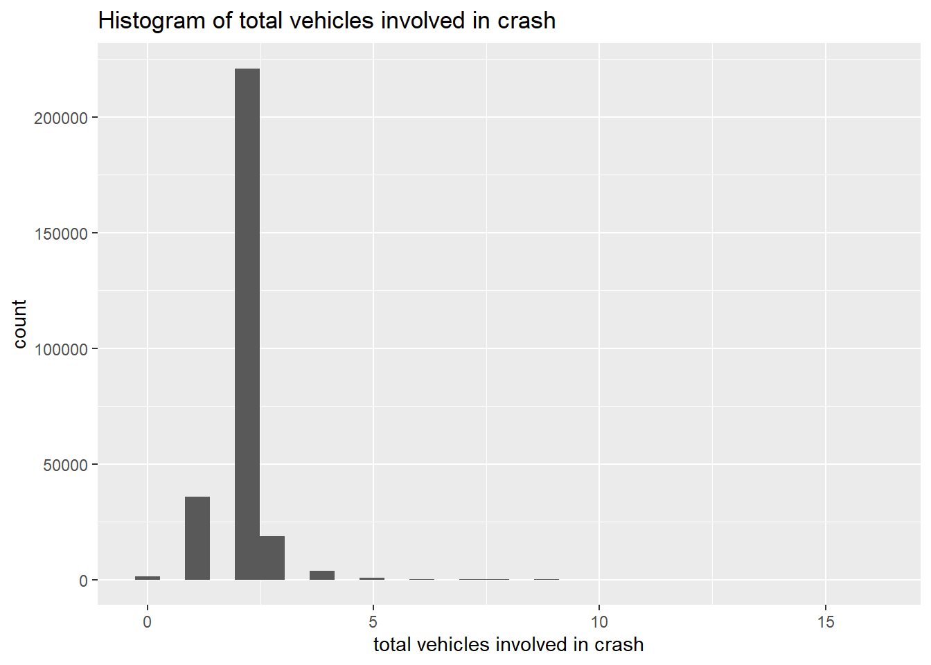
You should now have enough basics to be able to write functions on your own. I strongly encourage you to practice using them. They streamline both code and thinking, and they are the key to programming efficiently and reliably.
G. Homework
- In section B.1., why do
summer(x = 1, y = 2)
summer(x = 2, y = 1)
not yield the same output? Write in math what each one does.
In section C.1., why does the call
summer3(x = 5, y = 3)return a value whensummer2(x = 5, y = 3)does not?In C.2., why does
summer(x = "fred", y = "ted")yield an error?Fix the function in part F to remove the graph background. In
ggplotwe remove the grey background by adding to the theme element:
plotto <- ggplot() +
  geom_whatever(data = df,
                mapping = aes(x = var, y = yvar)) +
  theme(panel.background = element_blank())
You can also get rid of the gridlines with
  theme(panel.background = element_blank(),
        panel.grid.major = element_blank(),
panel.grid.minor = element_blank())- Make a function that automates a graphics operation of interest to you, using a dataset not from this tutorial.