library(quarto)Tutorial 10: Presenting Work Using Quarto
In our final week, we are turning to how to make presentations or webpages with work you’ve already created in R. We do this with a very new package called quarto. This package allows you to write code in a text file to create web books, such as this tutorial book. You can also make presentations, such as the ones I make for class on how to do things in R.
My opinion is that quarto is very simple to start, and that it is great if you are ok with the basic templates it offers. In my experience, quarto is not very flexible outside of the templates. I’ve also found it somewhat buggy in creating presentations. All that said, it is incredibly easy to get started, and I think the basic templates look pretty good.
In today’s tutorial, we’ll first make a short presentation. Then we’ll make a very short book and that you can open on your computer.
Unlike the other tutorials this semester, this is the first outing for this tutorial. In other words, this tutorial is new, and quarto is also new. Please let me know any problems you run into as quickly as you can and I will endeavor to fix rapidly.
A. Getting to know quarto a bit
In this section, we’ll discuss what quarto is and look at some quarto examples. This will help give you a sense of the possibilities for use.
A.1. What is quarto?
As I understand it (though you can see the official description here), quarto aims to be a product that links programming and output. For example, when I write an academic paper, I may program the analysis in R, make jpgs in R, and make final tables in another software. Then you might write the final paper in MSWord (I generally use Latex via Overleaf).
quarto aims to get rid of all of these intermediate steps and be the sole place where you do all your writing – the code, the output and the text. I wouldn’t say that it yet serves that purpose for me, but I have found it to be a very good tool for creating web documents that use R.
quarto is created by the authors of RStudio, who renamed themselves Posit when they released quarto. quarto is designed as a replacement for R Markdown, which tried to do these things for R. However, quarto can work with not just R but Python and other languages and inputs, such as Jupyter notebooks.
For your purposes, it is probably best to think of quarto as another package in R that can help you produce web and presentation output. Rather than writing just in R code, you’ll write regular text and R code, along with some special markers in mark-up code.
A.2. For presentations
You can find example presentations here. When I present on how to code in R, I am using a quarto presentation.
These presentations are in reveal.js, which is a web format. This means that any product that can read html documents – namely a web browser – can open your slides.
A.3. For web books
quarto can also create a web book. This is basically a webpage, but with built-in chapters on the left and sections at the right. See examples here. The tutorials for this class are presented in a quarto book.
B. Install quarto
Make sure that you are using a RStudio version v2022.07 or later. Don’t know what version you’re using? Go to the Help menu, and choose “About RStudio.”
Posit strongly recommends that you use RStudio v2023.03 or later. If you installed RStudio at the beginning of this semester, you are probably already out of date!
Make your life easier and update your RStudio. quarto is new and can be buggy, so I think this is a wise investment. Go here and install the latest RStudio and then come back.
Now see if quarto is installed by typing
If you don’t have quarto installed, do
install.packages("quarto")C. Create a short presentation
In this section we’ll make a very basic presentation with three slides, and then add a fourth. If you would like to see what the three slide version looks like, follow this link.
C.1. Create the presentation document
Start your presentation by going to the File menu: File \(\rightarrow\) New File \(\rightarrow\) Quarto Presentation.
You should see a window that looks like 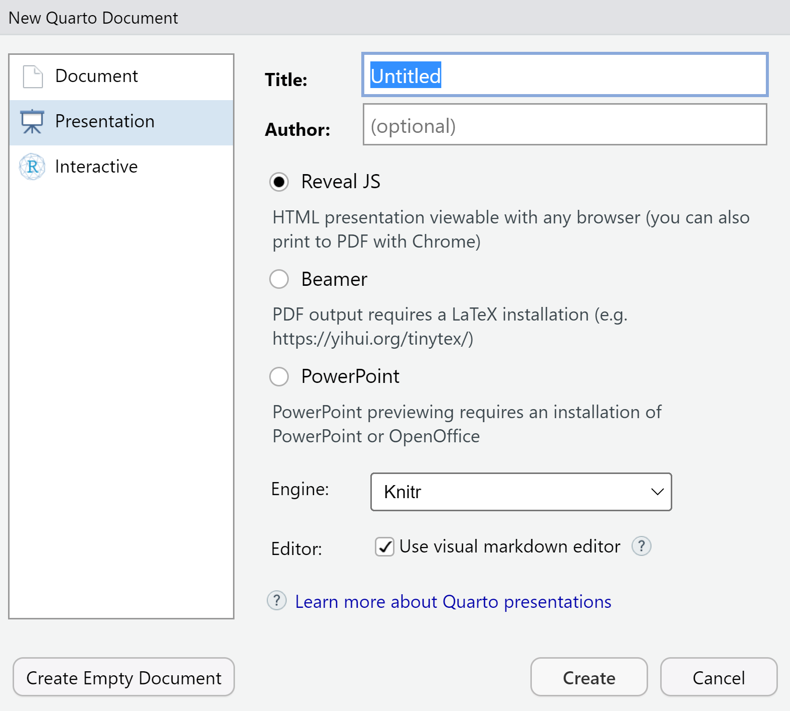
Make the title whatever you’d like. You can fill in the author section or not. To make a presentation, you should keep the selection button on “Reveal JS”. The other two options create a pdf (Beamer), or power point. Leave the engine as knitr and to start, uncheck the “visual markdown editor.”
After you click what do you click?, you should see a new document open up that looks like this 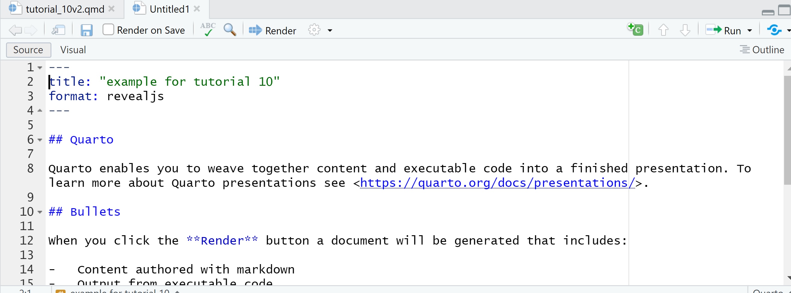
Save this document! Save it somewhere you’ll remember. When you save this document, don’t add an extension. RStudio will automatically save it with a .qmd extension. This extension is the same for all quarto documents.
C.2. Look at the presentation document
The presentation document you have open has two parts. The top part is the YAML header and should look like what’s pasted below. YAML stands for “yet another markup language.” This is the part of the document that tells the compiler (the thing that takes the text you type into an output format) what to do.
---
title: "example for tutorial 10"
format: revealjs
---
This YAML header has only two elements. The first has the title that you typed in when you created the document. The second line tells the format: reveal.js.
Every quarto document has a YAML header. We’ll see how this header is different when we go to make the book in section E.
After the YAML header, you’ll see a section that already has some text. Note that the three back ticks under ## Code are not and should not be preceded by a \ – but I can’t figure out how to get this to show up without it. Apologies! This will be a lingering issue for the rest of this tutorial.
## Quarto

Quarto enables you to weave together content and executable code into a finished presentation. To learn more about Quarto presentations see <https://quarto.org/docs/presentations/>.

## Bullets

When you click the **Render** button a document will be generated that includes:

-   Content authored with markdown
-   Output from executable code

## Code

When you click the **Render** button a presentation will be generated that includes both content and the output of embedded code. You can embed code like this:

\```{r}
#| eval: true
#| echo: true
df <- data.frame(v1 = c(1,2,3),
                 v2 = c("a","b","c"))
df
\```
This part of the document – everything below the YAML header – shows up in the final presentation. The ## denote slide titles, and each ## starts a new slide. The text below the ## is the text that appears on the slide.
Of course, this document does not look like slides. In the next sub-section, we’ll go from this document to slides.
C.3. Render the presentation document
To go from the .qmd document to slides that you can see in a web browser, you need to “render” the slides. At the top of the document, there is a “render” button – see the highlight below 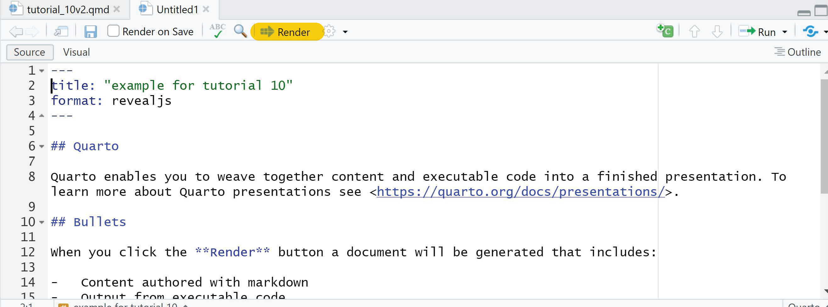 .
.
Press the “render” button and R will do some blah blah blah in the “background jobs” window. Then you should see a web browser pop up. The first slide should have the title you had in the YAML header.
Mine looks like 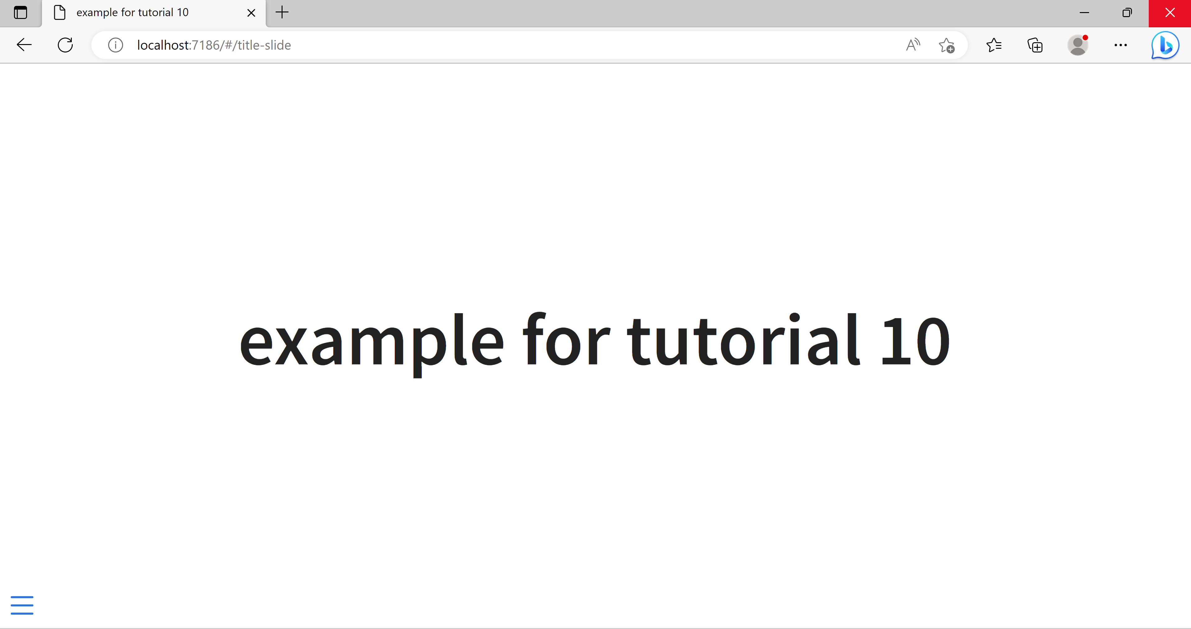
You can then use your keyboard arrows to go through the slides. As you look at the slides, go back and forth between the slides in the web browser and the text in your qmd document. This will allow you to see what code creates the look on each slide.
C.4. Slide elements
Now we will go through the elements in the .qmd document that create the slides. You already know about the YAML header that tells the compiler what the format of the document is.
Notice that each slide has a title and that the title is the word on the same line as the ##. For example, in the first document, the code for the slide title is
## QuartoThe text after this title says
Quarto enables you to weave together content and executable code into a finished presentation. To learn more about Quarto presentations see <https://quarto.org/docs/presentations/>.This is the text that appears on the slide. The last url is a link – which is in blue in the presentation. The <> that surrounds the url make it into a link, as a well as an address that shows up in the slide.
The code for the second slide of the presentation is
## Bullets

When you click the **Render** button a document will be generated that includes:

-   Content authored with markdown
-   Output from executable code
You’ve already seen the slide title – here “Bullets”. There are two new types of notation on this slide. The first is the ** that surround the word “Render.” This makes Render in bold.
The second important quarto notation on this slide is the bullets. You’ll see that on the “Bullets” webpage, there is a short bulleted list: 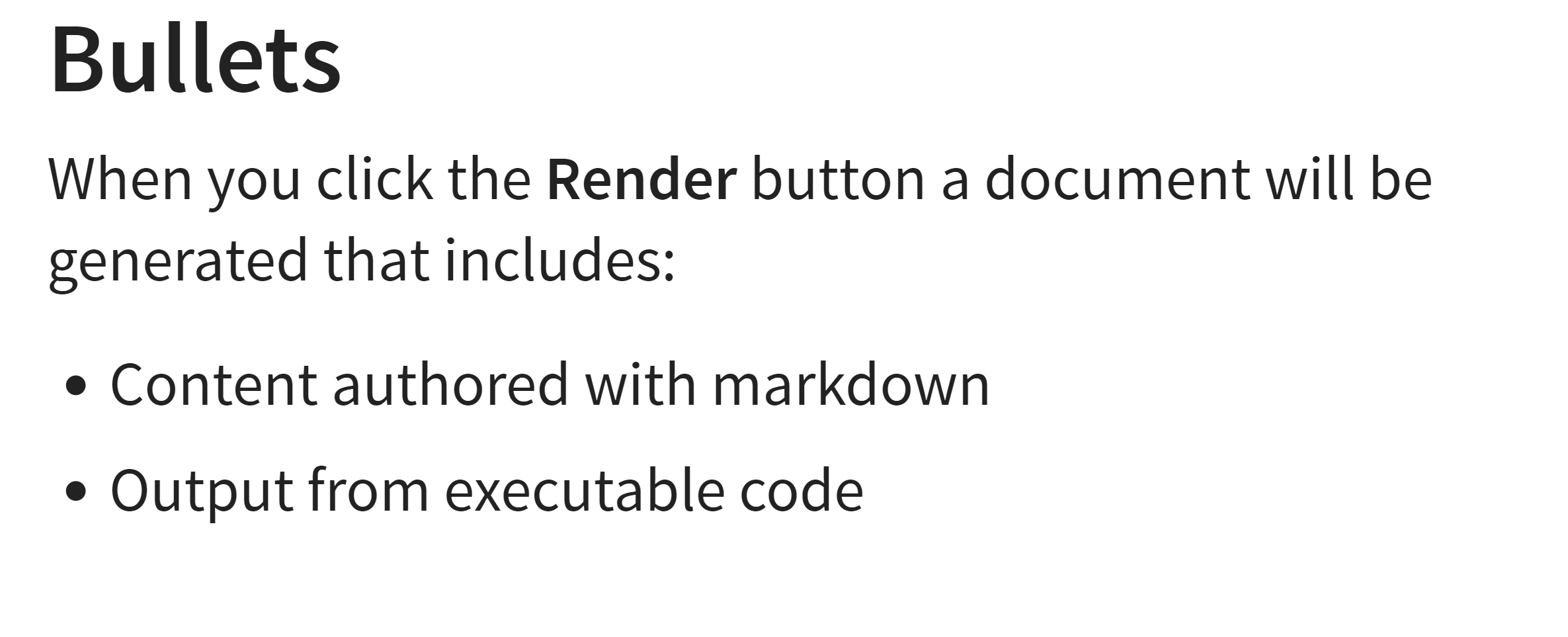
In the .qmd text, each bullet point is a dash -.
The final slide in this presentation is the Code slide. This slide shows you how to include R code. We’ll go into more detail in the next section about this.
C.5. Edit the presentation document
To get started, let’s add a slide to this presentation document. To do this, you need to add ## and a title of the slide, and some text for the slide.
Here’s what I’m adding to the presentation slides.
## A New Slide

1. Learn R
2. Make webpage

\```{r}
#| eval: true
#| echo: true
df <- data.frame(v1 = c(1,2,3),
                 v2 = c("a","b","c"))
df
\```
Type this new content into your presentation document, recalling that neither the ```{r} nor the closing backs should have a backslash in front. Save and render again. You should see a new webpage. You should now have four slides, rather than three. My final slide looks like the 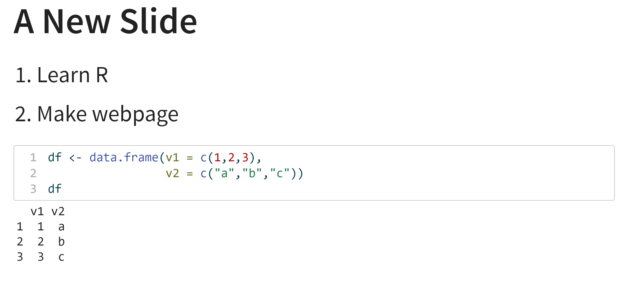 .
.
Let’s unpack the code here. First, the numbered list creates a numbered list. Then the next part is the way you create R code. To get R code to look like code, you start with three back ticks, then curly braces, the letter r and closing curly braces. On my keyboard, the back tick that is at the top left of the keyboard. End the code block with three more back ticks. Remember that these lines should not have a \ preceding them when you type them in your .qmd – it’s a quarto presentation problem I can’t figure out.
quarto interprets everything you put into a code block with r in the curly braces as R code. I have two options here for the code block (or chunk) in the first two lines:
#| eval: false
#| echo: true
The first means that quarto should evaluate the code in the block. The second means that R should print the commands, in addition to the output, to the html output file.
D. General quarto commands
Now that we’ve had an overview of quarto, we’ll go into a more systematic review of the types of things you can do.
D.1. Dividing a document
In a presentation, ## denotes a slide title.
In a book, #, ##, ###, etc. are section headers. In this document, this section D.1. is denoted by the header ### D.1. Dividing a document.
I have not figured out how to auto-number the sections, so I manually number them (this is awful!).
D.2. Changing text: bold, italics and other
You can tell quarto to change the font to bold using **bold**, and to italics as *italics*.
D.3. Columns
In some of my presentations, I have found it helpful to have a two-column layout. Here’s how I make columns in this presentation:
:::: columns
::: {.column width="65%"}
::: {.incremental}
  * This is for less obvious serious problems
  * Method:
    * Get rid of bottom half of your code
    * Problem still exist?
    * Get rid of bottom half of your code
    * Problem still exist?
    * etc..
:::
:::

::: {.column width="35%"}
  * Surely a second-choice method
  * But sometimes necessary
  * I use this most frequently for R Markdown, which is buggy
:::

::::
The :::: columns indicates to quarto that you want to start a set of columns, and :::: indicates when quarto should end the columns.
Within those markers, each column begins and ends with :::. At the beginning of the column, you can specify the width with {.column width="xx%"}, where xx is a percentage, and where all the percentages should add up to 100%. Don’t use spaces before or after the equals sign, or this will fail!
D.4. Including images
If you are creating images in R, you can simply type the name of the image inside a R code block. For example, suppose you used ggplot to create a histogram called leah.hist. To have leah.hist appear in a presentation window, you need only type leah.hist inside a code block.1
For images that are files on your computer, write code like this  or .png, or whichever supported file type you use.
You can change the width of the image with text after the code that includes the image. For example, you can write {width=70%}.
You can also specify the width in pixels ({width=300}), or inches ({width=6in}).
At the moment, quarto cannot add an image file that sits on a network drive and not in the same directory as the presentation. This is a known bug, but it has not yet been fixed. So I suggest that you put all the images you’d like to include in the same directory as your .qmd file.
D.5. Options for R code blocks
There are many options for the code you include in your qmd document. I’ll discuss options for naming each code chunk and for modifying the output of code chunks. This, however, just scratches the surface of what R can do. There are additional options for annotating code chunks, and you can make code fold, add line numbers and much more.
All code chunk options go below the ```{r} and begin with #|.
I encourage you to give a name to each code chuck that you include. This allows you to refer within the document to each code chunk, but is probably most useful for debugging. For example, to name a chunk “first-chuck” you would add #| label: first-chunk.
I frequently use the options to show output. A full list is here, and I’ll briefly review the options I find most useful here.
#| eval: true/falseWhen true,quartoexecutes the code in the block. When false,quartodoes not execute the code. If you want to show code that generates an error, settingevalequal to false is a good idea. If true, the code will break during compiling and you won’t have a final document.#| echo: true/falseWhen true,quartowrites code to the html output. When false,quartoshows any output, such as numbers or figures, but doesn’t write the code itself to the html output. If I want to show a R-created figure, I often useeval: trueandecho: false.#| warning: true/falsewhen false, R omits printing warning messages from your code to the html output. When true, R includes warnings. I usually setwarning: falsewhen I show code loading packages to students.#| error: true/falseWhen true, errors print in the html output, but do not stop the code from processing. When false, which is the default, errors stop the code from processing.
D.6. How quarto compiles
A few words of warning on how quarto processes. quarto starts at the top of your document and works forward. If it hits an error it can’t resolve, it stops and does not generate an output file. You will see error messages in the “Background Jobs” window.
Suppose you learn that there is an error in your third R chunk. Your first inclination might be to go to that chunk in your .qmd document and run it (with the little green arrow at the top right of the chunk). However, if that chunk relies on information from previous chunks – perhaps a dataframe you created in a previous chunk – you’ll need to re-run all the previous chunks to get your chunk ready for testing.
Because this is so annoying, I generally write code in a R file (a .R script). When that code works, I then plug it into a quarto document, diving up into chunks as I see fit.
D.7. How to open your presentation
RStudio automatically opens up your presentation when you render it. However, if you’d like to open it without pushing the render button, you can find the presentation files in the same directory as your .qmd file. The file has the same name, but a .html extension. I can’t see the extension in my file explorer, but my file has the icon of a web browser.
To open the presentation file, open a web browser window and navigate to where the .html file is and open it.
If you want to move the presentation file, you need to move the .html file and the folder by the same name. This folder has a lot of little files in it that quarto creates to make the webpage look nice. If you move the html file, but not these extra files, the webpage may not load, or will load and look awful.
D.8. Other things you can do
There are many many other things you can do in a quarto document, most of which I don’t know exist. Here is a limited list of some additional possibilities:
- Add a search bar
- Make nested lists
- Make a pdf output from the webpage
- Add colors
And many many more. See the ever-evolving quarto documentation for more information.
D.9. Web hosting
To put your quarto page up on the internet – something we will not do today – you have two options. The fastest and cheapest is to make yourself a github page and host your page there. I haven’t done this, but there are lots of instructions on how to do this online.
The second option is why I do. I pay a webhosting company, buy a domain name (www.leahbrooks.org) and put my pages on this website.
E. Write and compile a book
You’ve already created a presentation. Now we’ll briefly review how to make a web book, just like the one I have created for the tutorials for this class.
E.1. Create a book file
Start by going to File \(\rightarrow\) New Project \(\rightarrow\) Quarto Book.2 (Choosing “new file” will not work here – you’ll get a html document, not a book.)
I strongly recommend that you choose “new directory” at the window below, as this book should sit in its own directory, alone.
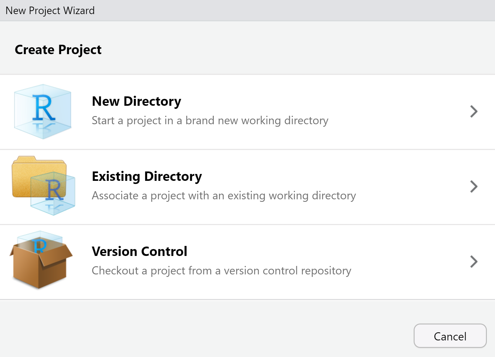
For “project type,” choose “quarto book.”
Then on the next screen, create a name for your new directory. For purposes of this class, uncheck the “visual” option on this menu. Then select “open in new session” and click “create project.” 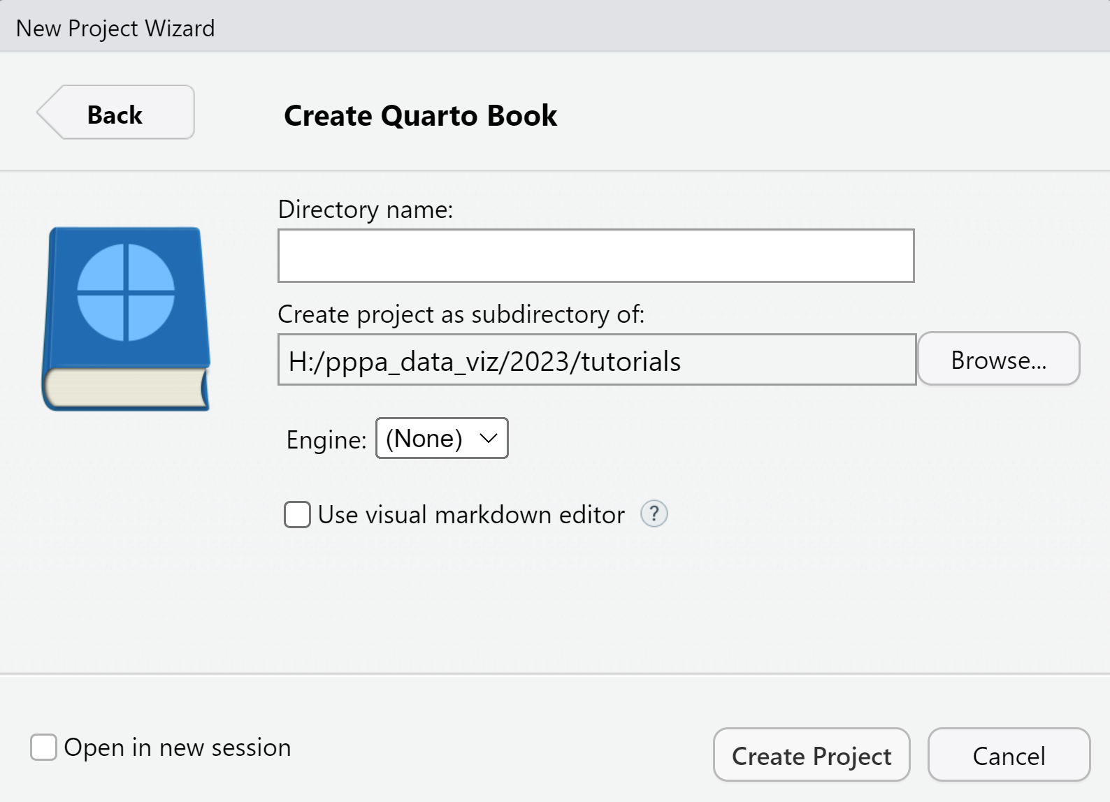
If you now look at the files on your computer, you should find a new directory named as you requested. Inside this directory, you’ll find a bunch of files. You should see 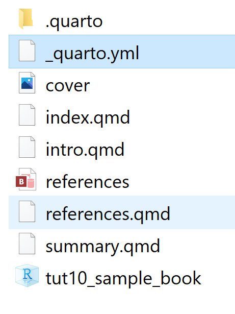
E.2 Explore the book file YAML
What makes a book different from a presentation or webpage is that it has its YAML header in a separate document. Open up _quarto.yml in RStudio.
Here is what I see in the default _quarto.yml file:
project:
  type: book

book:
  title: "tut10_sample_book"
  author: "Jane Doe"
  date: "4/23/2023"
  chapters:
    - index.qmd
    - intro.qmd
    - summary.qmd
    - references.qmd

bibliography: references.bib

format:
  html:
    theme: cosmo
  pdf:
    documentclass: scrreprt
The indenting in this text is not decorative. Here, indenting has content, so that “chapters” are a subset of “book.” Similarly, “html” is a subset of “format,” and the theme of the html is “cosmo.”
This YAML makes a book with four “chapters.” You list any chapters you want to include under the chapters: heading. By default, we start with index.qmd, intro.qmd, summary.qmd, and references.qmd. Note that each of these four chapters has a .qmd file already created.
Don’t rename or delete index.qmd. This is the landing page for your webpage. For the rest, you can re-name chapters as you please. If you want to do this, you need to do two things: make a file with [chapter_name].qmd and put [chapter_name].qmd in the list of chapters for your book.
This YAML file is also where you can make all kinds of changes that will impact the entire document – colors, fonts, spacing, search bar – none of which we cover today.
E.3. Explore the remaining book files
Open index.qmd, which looks like
# Preface {.unnumbered}

This is a Quarto book.

To learn more about Quarto books visit <https://quarto.org/docs/books>.
To modify the book landing page, edit this file, using all the quarto tricks we’ve already covered.
E.4. Populate one chapter
Let’s add one chapter to this book. This requires two operations: adding a .qmd file for the chapter and adding the chapter to the YAML file.
To make a new .qmd for the chapter, in the directory where you book is, open intro.qmd. Then do “File” \(\rightarrow\) “Save As” and save this file as chapter_1.qmd. When adding new chapters, do not put spaces in your file names. Spaces are likely going to cause errors.
In your new file, write a new chapter title after the #, and write a few lines of new text. Here’s my new chapter_1.qmd:
# The Very Lovely Chapter 1
I say many things.
And I have a picture, courtesy of Wassily Kandinsy and the [Phillips Collection](https://www.phillipscollection.org/collection/succession).
The picture I include is in the same directory as the .qmd file. This new chapter not work for you, unless you have a png file named 20230423_kandinsky.png in the same directory as the book.
Now we edit the YAML file to add this chapter. The only part you need to edit is the lines under the book: heading. Initially, this looked like
book:
  title: "tut10_sample_book"
  author: "Jane Doe"
  date: "4/23/2023"
  chapters:
    - index.qmd
    - intro.qmd
    - summary.qmd
    - references.qmd
Edit the file so it looks like
book:
  title: "tut10_sample_book"
  author: "Jane Doe"
  date: "4/23/2023"
  chapters:
    - index.qmd
    - intro.qmd
    - chapter_1.qmd
    - summary.qmd
    - references.qmd
E.5. Render the book
Rendering a book is slightly more complicated than rendering a presentation (or a single webpage). With a presentation, everything is in one single .qmd document.
With a book, this is not the case. You can render individual pages, but if you make overall changes in the YAML file, these may not be reflected unless you render the entire book.
To render a book, I have found these steps below to be foolproof. While they are slightly more complicated than in the quarto documentation, I have had trouble with the documentation commands.
Start by typing
getwd()in the console.
R will report the “working directory” you are in. This is the place R will look for files to compile. For the R book I’ve made for this example, R tells me
> getwd()
[1] "H:/pppa_data_viz/2023/tutorials/sample_quarto_products_tutorial10/tut10_sample_book"
This is the file where my _quarto.yml file is for the book, so I am set. But if the directory R lists is not where your file is, then type the command below, putting the full path of your book directory in.
setwd("path where your file is")You can check whether this command worked by doing getwd() again.
Now that you’re in the right directory, let’s compile the book. Type
quarto::quarto_render()in the console. You don’t have to specify a file name, because RStudio knows that all files in the working directory may be associated with the book, as directed by the info in the .yml document.
There will be a lot of blah blah blah in the Background Jobs window, and the processing, even for this small file, may take quite a while.
When the progress bar tells you you’re done, and if the book doesn’t auto-open in a new window, you can open the file yourself by going to a web browser and directly opening the file (ctrl + f on a pc). Navigate to the directory where your book is and then one directory further into the directory _book. Now choose index.html, and you should see the home page of your book. You should be able to navigate to all the pages of the book through the menu at the left.
You can find my sample book here
F. Many other options and possibilities
There are millions of additional options for everything quarto. For books, see some of them here.
More broadly, everything is modifiable to some degree. You can find full documentation at https://quarto.org.
I expect that quarto should improve appreciably over the next year or two. It was only released in July 2022, so there remains lots of opportunity for users to test and modify and improve.
G. Homework
Make a presentation using quarto with
- a bulleted list with two levels
- a figure
- R code and a R figure
To turn this in, create a sub-folder in your google folder for this tutorial. Put the .html file and the associated folder in this google drive folder.