install.packages("sf", dependencies = TRUE)Tutorial 5: Maps 1 of 2
This is our first of two tutorials on maps, concentrating on the R package sf. This tutorial introduces digital maps. It then gives examples of how to present them, followed by some examples of the type of spatial analysis you can do with this package. In our second mapping class, we concentrate on choropleth maps.
This tutorial begins by showing you how to make a simple map, and it ends with relatively sophisticated programming showing you how to count points within polygons. Specifically, here are the steps you’ll take
- Load the package you’ll need
- Draw map of DC wards, label the wards, and add a map of DC school administration buildings
- Apply these techniques with bigger point data
- Count points in polygons
In addition to these goals, you will also learn how to download data from an application programming interface (API). This is a great way to grab data that becomes even better as you want to do repetitive tasks; we’ll talk more about repetitive tasks later in the semester.
While making this tutorial, I consulted three online tutorials that I would recommend if you want more in-depth coverage of specific map issues. See
- The University of Chicago’s Computing for the Social Sciences
- The authors of the the package, in-depth, but sometimes difficult to follow
- A random guy
A. Load packages
This week are are adding a new package to our repetoire: sf. This package is a quantum leap forward for mapping in R. It is fast and, relative to what was previously available, easy to use (you may not believe this after today’s tutorial, but it is true). This package is also designed to work with ggplot, so today’s lesson shows you how these packages integrate.
As a word of warning, sf is very new. As such, the online help is not as extensive as for ggplot, and every so often you run into odd errors, or things that you think the package should do but does not. Despite all this, we are learning it because I think it’s the best for mapping and spatial analysis in R: comprehensive and fast.
All sf commands begin with st_, as you’ll see in this tutorial. We introduce only a fraction of what sf can do in this tutorial, so look at the online help or discuss with me if you have more questions.
Begin by installing the sf package, using the dependencies = TRUE option. This option automatically installs any packages that sf needs that you don’t have. Install this package once (and for all) by typing the install.packages() directly into the console window.
You will also need an additional package that will help you get from the file type you download to the to the kind of map file that we are using this class. This package is called geojsonsf, and please install it as below
install.packages("geojsonsf", dependencies = TRUE)Everything else in this tutorial should be written in a R script.
We also load tidyverse – a package you’ve already installed. Here I use the require() command. This command checks if you have the package. If you do, it loads the package. If it doesn’t it downloads the package and then loads the package.
Now load the packages we’ll need for today. Remember that these lines go directly into your R script.
require(sf)Loading required package: sfLinking to GEOS 3.9.1, GDAL 3.3.2, PROJ 7.2.1; sf_use_s2() is TRUErequire(tidyverse)Loading required package: tidyverse── Attaching packages ─────────────────────────────────────── tidyverse 1.3.1 ──✔ ggplot2 3.3.6 ✔ purrr 0.3.4
✔ tibble 3.1.7 ✔ dplyr 1.0.9
✔ tidyr 1.2.0 ✔ stringr 1.4.0
✔ readr 2.1.2 ✔ forcats 0.5.1── Conflicts ────────────────────────────────────────── tidyverse_conflicts() ──
✖ dplyr::filter() masks stats::filter()
✖ dplyr::lag() masks stats::lag()require(geojsonsf)Loading required package: geojsonsfWarning: package 'geojsonsf' was built under R version 4.2.1B. Load, explore and plot two shapefiles
In this section we load a shapefile of DC wards, label them, and plot one additional feature on top of the ward maps.
B.1. Load
We begin by loading a shapefile of wards in DC. There are 8 wards in DC. Wards are electoral districts for councilmembers (there are also 5 at-large councilmembers). Thus we expect this file to have 8 polygons. You can download this file from DC’s Open Data site here. From the download menu, choose “shapefile” and then save in a location you’ll remember. If you don’t choose the shapefile format, nothing below will work.
To load a shapefile into R with sf, you use the st_read() command. You tell R where the file is, and what type of file it is by the extension.
The st_read() command is specifically designed to work with shapefiles, which are files that contain spatial data. For more details on such files, see the lecture notes.
Begin by loading the data, as below.
dc.wards <- st_read("H:/pppa_data_viz/2019/tutorial_data/lecture05/Ward_from_2012/Ward_from_2012.shp")Reading layer `Ward_from_2012' from data source
`H:\pppa_data_viz\2019\tutorial_data\lecture05\Ward_from_2012\Ward_from_2012.shp'
using driver `ESRI Shapefile'
Simple feature collection with 8 features and 82 fields
Geometry type: POLYGON
Dimension: XY
Bounding box: xmin: -77.1198 ymin: 38.79164 xmax: -76.90915 ymax: 38.99597
Geodetic CRS: WGS 84Note that sf tells you a little about this file immediately upon loading. The “8 features” to which R refers are the 8 wards, so features are the geographic units of analysis. We also learn that the “geometry type” is this file is polygons (not lines or points). R also tells us maximum and minimum latitude and longitude of the map and the projection number (more on this later).
You have now loaded a shapefile, and specifically a shapefile in the “simple features” format (other formats include geoJSON and sp).
B.2. Explore
One of the useful aspects of simple features is that you can use all your usual dataframe commands on them.
First try
head(dc.wards)Simple feature collection with 6 features and 82 fields
Geometry type: POLYGON
Dimension: XY
Bounding box: xmin: -77.08172 ymin: 38.79164 xmax: -76.90915 ymax: 38.9573
Geodetic CRS: WGS 84
OBJECTID WARD NAME REP_NAME
1 1 8 Ward 8 Trayon White, Sr.
2 2 6 Ward 6 Charles Allen
3 3 7 Ward 7 Vincent Gray
4 4 2 Ward 2 Jack Evans
5 5 1 Ward 1 Brianne Nadeau
6 6 5 Ward 5 Kenyan McDuffie
WEB_URL REP_PHONE
1 http://dccouncil.us/council/trayon-white-sr (202) 724-8045
2 http://dccouncil.us/council/charles-allen (202) 724-8072
3 http://dccouncil.us/council/vincent-gray (202) 724-8068
4 http://dccouncil.us/council/jack-evans (202) 724-8058
5 http://dccouncil.us/council/brianne-nadeau (202) 724-8181
6 http://dccouncil.us/council/kenyan-mcduffie (202) 724-8028
REP_EMAIL REP_OFFICE WARD_ID
1 twhite@dccouncil.us 1350 Pennsylvania Ave, Suite 400, NW 20004 8
2 callen@dccouncil.us 1350 Pennsylvania Ave, Suite 406, NW 20004 6
3 vgray@dccouncil.us 1350 Pennsylvania Ave, Suite 406, NW 20004 7
4 jevans@dccouncil.us 1350 Pennsylvania Ave, Suite 106, NW 20004 2
5 bnadeau@dccouncil.us 1350 Pennsylvania Ave, Suite 102, NW 20004 1
6 kmcduffie@dccouncil.us 1350 Pennsylvania Ave, Suite 506, NW 20004 5
LABEL AREASQMI Shape_Leng Shape_Area POP_2000 POP_2010 POP_2011_2 POP_BLACK
1 Ward 8 11.937871 28714.07 30965852 74049 73662 81133 75259
2 Ward 6 6.221045 24157.98 16064917 70867 76238 84290 29909
3 Ward 7 8.809914 22345.23 22818183 69987 71748 73290 69005
4 Ward 2 8.684517 29545.80 22492798 63455 76645 77645 6817
5 Ward 1 2.535896 12925.38 6567941 71747 74462 82859 25110
6 Ward 5 10.390304 22893.40 26910761 71440 74308 82049 57733
POP_NATIVE POP_ASIAN POP_HAWAII POP_OTHER_ TWO_OR_MOR NOT_HISPAN HISPANIC_O
1 110 310 12 711 872 79843 1290
2 295 3573 40 1233 2529 79000 5290
3 219 225 17 1211 908 70987 2303
4 213 7640 30 2496 2875 69529 8116
5 300 3509 111 6259 2596 65755 17104
6 335 1622 9 3758 1915 75058 6991
POP_MALE POP_FEMALE AGE_0_5 AGE_5_9 AGE_10_14 AGE_15_17 AGE_18_19 AGE_20
1 35573 45560 7879 7061 5963 3596 2945 1800
2 40411 43879 4779 2747 2235 1088 1370 794
3 33916 39374 5230 4485 4333 2944 2162 1347
4 39214 38431 2173 1110 571 486 6200 3363
5 41368 41491 4733 2644 1934 1223 2399 1613
6 38692 43357 5778 3972 2654 2249 2817 1533
AGE_21 AGE_22_24 AGE_25_29 AGE_30_34 AGE_35_39 AGE_40_44 AGE_45_49 AGE_50_54
1 1748 4070 6306 5951 4617 4873 4429 4978
2 724 4596 13427 12512 8052 5474 4524 4350
3 1107 3170 5036 5083 4154 5166 4794 5715
4 3485 6463 12614 10475 6491 4175 3445 3413
5 1642 5487 15600 12286 7378 5099 4784 3963
6 1531 3882 8514 7439 5996 5228 4828 4905
AGE_55_59 AGE_60_61 AGE_65_66 AGE_67_69 AGE_70_74 AGE_75_79 AGE_80_84
1 5001 1578 1011 1211 1904 1026 634
2 4724 1830 1518 1596 2167 1522 816
3 5272 1716 1254 1680 2370 1719 1290
4 3248 1447 1214 1325 1763 764 724
5 2618 1420 802 1208 1778 954 505
6 5274 1736 1108 1640 2361 2079 1947
AGE_85_PLU MEDIAN_AGE UNEMPLOYME TOTAL_HH FAMILY_HH PCT_FAMILY
1 432 29.3 22.9 29470 17747 60.2205632846963
2 958 33.9 6.3 40100 15110 37.6807980049875
3 1142 37 19.1 29266 15574 53.2153352012574
4 863 30.9 3.7 38870 9071 23.3367635708773
5 738 31.3 6.6 34907 12253 35.1018420374137
6 2135 35.4 14.1 31656 14893 47.0463735152894
NONFAMILY_ PCT_NONFAM PCT_BELOW_ PCT_BELO_1 PCT_BELO_2 PCT_BELO_3
1 11723 39.7794367153037 37.7 35.3 10.8 38.8
2 24990 62.3192019950125 12.5 9.6 4.5 25.7
3 13692 46.7846647987426 27.2 23.6 8.9 28
4 29799 76.6632364291227 13.4 4.7 10.1 33.2
5 22654 64.8981579625863 13.5 11 7.7 23.3
6 16763 52.9536264847106 19 13.5 12.5 20.4
PCT_BELO_4 PCT_BELO_5 PCT_BELO_6 PCT_BELO_7 PCT_BELO_8 POP_25_PLU POP_25_P_1
1 54.1 21.6 0 51.2 36.4 <NA> 1858
2 13.9 11.6 0 10.7 6.2 <NA> 1785
3 12.8 5.3 0 19.7 20 <NA> 2259
4 26 23.5 0 12.6 10.3 <NA> 1743
5 8.7 6.9 0 26.8 11.5 <NA> 4324
6 19.1 17.7 0 27.9 10.4 <NA> 2796
POP_25_P_2 MARRIED_CO MALE_HH_NO FEMALE_HH_ MEDIAN_HH_ PER_CAPITA PCT_BELO_9
1 2614 <NA> 1886 11653 30910 17596 36.3
2 25882 <NA> 944 4157 94343 58354 6.3
3 3309 <NA> 1682 9499 39165 22917 22.9
4 28509 <NA> 458 754 100388 72388 13.5
5 22488 <NA> 1634 3133 82159 47982 17.9
6 11168 <NA> 1567 6726 57554 32449 21.6
PCT_BELO10 NO_DIPLOMA DIPLOMA_25 NO_DEGREE_ ASSOC_DEGR BACH_DEGRE MED_VAL_OO
1 10.8 5958 18736 10975 2149 3781 229900
2 4.5 3128 7079 6643 1852 19588 573200
3 8.9 6002 18683 10800 2569 4890 238900
4 10.1 988 2381 2980 940 16253 623500
5 7.7 3224 6984 5293 1258 17613 542100
6 12.5 5094 13788 11034 2196 11557 379800
Shape_Le_1 Shape_Ar_1 geometry
1 28714.07 30965852 POLYGON ((-76.97229 38.8728...
2 24157.98 16064917 POLYGON ((-77.0179 38.9141,...
3 22345.23 22818183 POLYGON ((-76.94186 38.9185...
4 29545.80 22492798 POLYGON ((-77.04946 38.9199...
5 12925.38 6567941 POLYGON ((-77.03523 38.9374...
6 22893.40 26910761 POLYGON ((-76.99144 38.9573...You can tell that this is a file with geographic data, rather than a usual dataframe, because the first lines of this file report that this is a simple feature file. The header also tells us that the features are polygons (second row), defined on x and y coordinates. The fourth line tells us the coordinates of a box that
Simple feature collection with 6 features and 10 fields
geometry type:  POLYGON
dimension:      XY
bbox:           xmin: -77.08172 ymin: 38.79164 xmax: -76.90915 ymax: 38.9573
geographic CRS: WGS 84
This shows some summary information on the geography part of the file – the type of features, the coordinate system – and then the first six rows of the data portion of the file.
We can also use str() to to get a description of all the variables. The geometry column at the end is where R hides all the geographic information.
str(dc.wards)Classes 'sf' and 'data.frame': 8 obs. of 83 variables:
$ OBJECTID : num 1 2 3 4 5 6 7 8
$ WARD : num 8 6 7 2 1 5 3 4
$ NAME : chr "Ward 8" "Ward 6" "Ward 7" "Ward 2" ...
$ REP_NAME : chr "Trayon White, Sr." "Charles Allen" "Vincent Gray" "Jack Evans" ...
$ WEB_URL : chr "http://dccouncil.us/council/trayon-white-sr" "http://dccouncil.us/council/charles-allen" "http://dccouncil.us/council/vincent-gray" "http://dccouncil.us/council/jack-evans" ...
$ REP_PHONE : chr "(202) 724-8045" "(202) 724-8072" "(202) 724-8068" "(202) 724-8058" ...
$ REP_EMAIL : chr "twhite@dccouncil.us" "callen@dccouncil.us" "vgray@dccouncil.us" "jevans@dccouncil.us" ...
$ REP_OFFICE: chr "1350 Pennsylvania Ave, Suite 400, NW 20004" "1350 Pennsylvania Ave, Suite 406, NW 20004" "1350 Pennsylvania Ave, Suite 406, NW 20004" "1350 Pennsylvania Ave, Suite 106, NW 20004" ...
$ WARD_ID : chr "8" "6" "7" "2" ...
$ LABEL : chr "Ward 8" "Ward 6" "Ward 7" "Ward 2" ...
$ AREASQMI : num 11.94 6.22 8.81 8.68 2.54 ...
$ Shape_Leng: num 28714 24158 22345 29546 12925 ...
$ Shape_Area: num 30965852 16064917 22818183 22492798 6567941 ...
$ POP_2000 : num 74049 70867 69987 63455 71747 ...
$ POP_2010 : num 73662 76238 71748 76645 74462 ...
$ POP_2011_2: num 81133 84290 73290 77645 82859 ...
$ POP_BLACK : chr "75259" "29909" "69005" "6817" ...
$ POP_NATIVE: chr "110" "295" "219" "213" ...
$ POP_ASIAN : chr "310" "3573" "225" "7640" ...
$ POP_HAWAII: chr "12" "40" "17" "30" ...
$ POP_OTHER_: chr "711" "1233" "1211" "2496" ...
$ TWO_OR_MOR: chr "872" "2529" "908" "2875" ...
$ NOT_HISPAN: chr "79843" "79000" "70987" "69529" ...
$ HISPANIC_O: chr "1290" "5290" "2303" "8116" ...
$ POP_MALE : chr "35573" "40411" "33916" "39214" ...
$ POP_FEMALE: chr "45560" "43879" "39374" "38431" ...
$ AGE_0_5 : chr "7879" "4779" "5230" "2173" ...
$ AGE_5_9 : chr "7061" "2747" "4485" "1110" ...
$ AGE_10_14 : chr "5963" "2235" "4333" "571" ...
$ AGE_15_17 : chr "3596" "1088" "2944" "486" ...
$ AGE_18_19 : chr "2945" "1370" "2162" "6200" ...
$ AGE_20 : chr "1800" "794" "1347" "3363" ...
$ AGE_21 : chr "1748" "724" "1107" "3485" ...
$ AGE_22_24 : chr "4070" "4596" "3170" "6463" ...
$ AGE_25_29 : chr "6306" "13427" "5036" "12614" ...
$ AGE_30_34 : chr "5951" "12512" "5083" "10475" ...
$ AGE_35_39 : chr "4617" "8052" "4154" "6491" ...
$ AGE_40_44 : chr "4873" "5474" "5166" "4175" ...
$ AGE_45_49 : chr "4429" "4524" "4794" "3445" ...
$ AGE_50_54 : chr "4978" "4350" "5715" "3413" ...
$ AGE_55_59 : chr "5001" "4724" "5272" "3248" ...
$ AGE_60_61 : chr "1578" "1830" "1716" "1447" ...
$ AGE_65_66 : chr "1011" "1518" "1254" "1214" ...
$ AGE_67_69 : chr "1211" "1596" "1680" "1325" ...
$ AGE_70_74 : chr "1904" "2167" "2370" "1763" ...
$ AGE_75_79 : chr "1026" "1522" "1719" "764" ...
$ AGE_80_84 : chr "634" "816" "1290" "724" ...
$ AGE_85_PLU: chr "432" "958" "1142" "863" ...
$ MEDIAN_AGE: chr "29.3" "33.9" "37" "30.9" ...
$ UNEMPLOYME: chr "22.9" "6.3" "19.1" "3.7" ...
$ TOTAL_HH : chr "29470" "40100" "29266" "38870" ...
$ FAMILY_HH : chr "17747" "15110" "15574" "9071" ...
$ PCT_FAMILY: chr "60.2205632846963" "37.6807980049875" "53.2153352012574" "23.3367635708773" ...
$ NONFAMILY_: chr "11723" "24990" "13692" "29799" ...
$ PCT_NONFAM: chr "39.7794367153037" "62.3192019950125" "46.7846647987426" "76.6632364291227" ...
$ PCT_BELOW_: chr "37.7" "12.5" "27.2" "13.4" ...
$ PCT_BELO_1: chr "35.3" "9.6" "23.6" "4.7" ...
$ PCT_BELO_2: chr "10.8" "4.5" "8.9" "10.1" ...
$ PCT_BELO_3: chr "38.8" "25.7" "28" "33.2" ...
$ PCT_BELO_4: chr "54.1" "13.9" "12.8" "26" ...
$ PCT_BELO_5: chr "21.6" "11.6" "5.3" "23.5" ...
$ PCT_BELO_6: chr "0" "0" "0" "0" ...
$ PCT_BELO_7: chr "51.2" "10.7" "19.7" "12.6" ...
$ PCT_BELO_8: chr "36.4" "6.2" "20" "10.3" ...
$ POP_25_PLU: chr NA NA NA NA ...
$ POP_25_P_1: chr "1858" "1785" "2259" "1743" ...
$ POP_25_P_2: chr "2614" "25882" "3309" "28509" ...
$ MARRIED_CO: chr NA NA NA NA ...
$ MALE_HH_NO: chr "1886" "944" "1682" "458" ...
$ FEMALE_HH_: chr "11653" "4157" "9499" "754" ...
$ MEDIAN_HH_: chr "30910" "94343" "39165" "100388" ...
$ PER_CAPITA: chr "17596" "58354" "22917" "72388" ...
$ PCT_BELO_9: chr "36.3" "6.3" "22.9" "13.5" ...
$ PCT_BELO10: chr "10.8" "4.5" "8.9" "10.1" ...
$ NO_DIPLOMA: chr "5958" "3128" "6002" "988" ...
$ DIPLOMA_25: chr "18736" "7079" "18683" "2381" ...
$ NO_DEGREE_: chr "10975" "6643" "10800" "2980" ...
$ ASSOC_DEGR: chr "2149" "1852" "2569" "940" ...
$ BACH_DEGRE: chr "3781" "19588" "4890" "16253" ...
$ MED_VAL_OO: chr "229900" "573200" "238900" "623500" ...
$ Shape_Le_1: num 28714 24158 22345 29546 12925 ...
$ Shape_Ar_1: num 30965852 16064917 22818183 22492798 6567941 ...
$ geometry :sfc_POLYGON of length 8; first list element: List of 1
..$ : num [1:3792, 1:2] -77 -77 -77 -77 -77 ...
..- attr(*, "class")= chr [1:3] "XY" "POLYGON" "sfg"
- attr(*, "sf_column")= chr "geometry"
- attr(*, "agr")= Factor w/ 3 levels "constant","aggregate",..: NA NA NA NA NA NA NA NA NA NA ...
..- attr(*, "names")= chr [1:82] "OBJECTID" "WARD" "NAME" "REP_NAME" ...A key attribute of a shapefile is its projection (for more on projections, see lecture notes). To find the projection of a sf file, use the st_crs() command. This reports the projection of the file.
# make sure it has a projection
st_crs(dc.wards)
Coordinate Reference System:
User input: WGS 84
wkt:
GEOGCRS["WGS 84",
DATUM["World Geodetic System 1984",
ELLIPSOID["WGS 84",6378137,298.257223563,
LENGTHUNIT["metre",1]]],
PRIMEM["Greenwich",0,
ANGLEUNIT["degree",0.0174532925199433]],
CS[ellipsoidal,2],
AXIS["latitude",north,
ORDER[1],
ANGLEUNIT["degree",0.0174532925199433]],
AXIS["longitude",east,
ORDER[2],
ANGLEUNIT["degree",0.0174532925199433]],
ID["EPSG",4326]]What does this information mean? There are (at least) two ways of identifying a projection. The first is the EPSG code. This is a numeric reference for the projection of the file. “EPSG” stands for the European Petroleum Survey Group, which first made this numeric system of reference. They have since been absorbed by the International Association of Oil and Gas Producers (IOGP). The IOGP maintains a registry of projections and associated codes that are very useful to anyone using spatial data.
The second method of identifying a projection is the “proj4string.” This is a set of characters and numbers that uniquely identify a projection. If at all possible, I prefer the EPSG codes, which are much easier to work with.
It’s useful to know the projection of a file if
- you’d like to do some analysis with that file and another shapefile – they should be in the same projection
- to know whether you’ve got the desired projection. For example, some US projections give a flat top to the US, and others give a curved top.
This particular projection is WGS84, a very standard projection maintained by the National Geospatial-Intelligence Agency, originating in the 1950s.
B.3. Plot
There are two major ways to generate a map plot from a sf file. You can use the plot command or ggplot. In the interests of time, we skip plot and head straight to ggplot, which is easier to manipulate and customize.
Using ggplot here is very similar to what we’ve already done. Instead of geom_bar() or geom_hist(), we now rely on geom_sf(). This command takes a simple feature as the data input and plots the polygons. Because we are plotting only the shape and no variables, there is no aes() portion of the command.
The below command is the simplest way to make a map from a “simple feature.” As we’ve done in previous tutorials with graphs, we create an object and then call it to see it. You could simply use ggplot without creating an object (though you wouldn’t be able to save it later if you wanted).
# two ways to plot -- second
ward.map <- ggplot() +
              geom_sf(data = dc.wards)
ward.map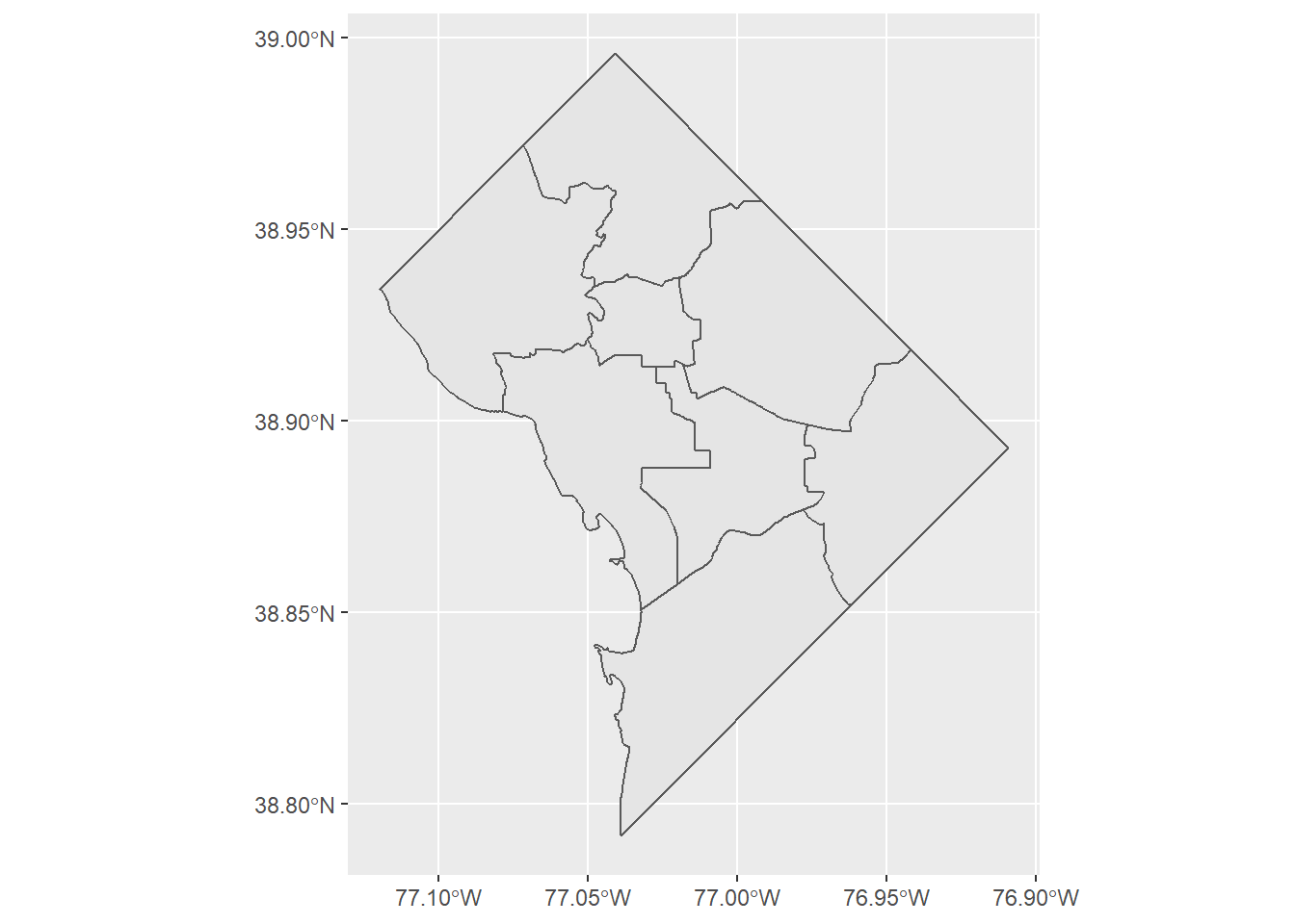
This is a basic map! You can use this same technique to plot any kind of shapefile you can download.
Of course, there are multiple things you might want to change on this map to make it more legible. Some basic modifications include the color of the polygon lines and the polygon fill. Below I set the color of the lines to pink and the fill to green. These commands are both inside the geom_sf() command, like graph options are inside geom_bar() or geom_histogram(). They are not inside the aes command because they are not based on data.
# with color and fill
ward.map <- ggplot() +
  geom_sf(data = dc.wards, color = "pink", fill = "green")
ward.map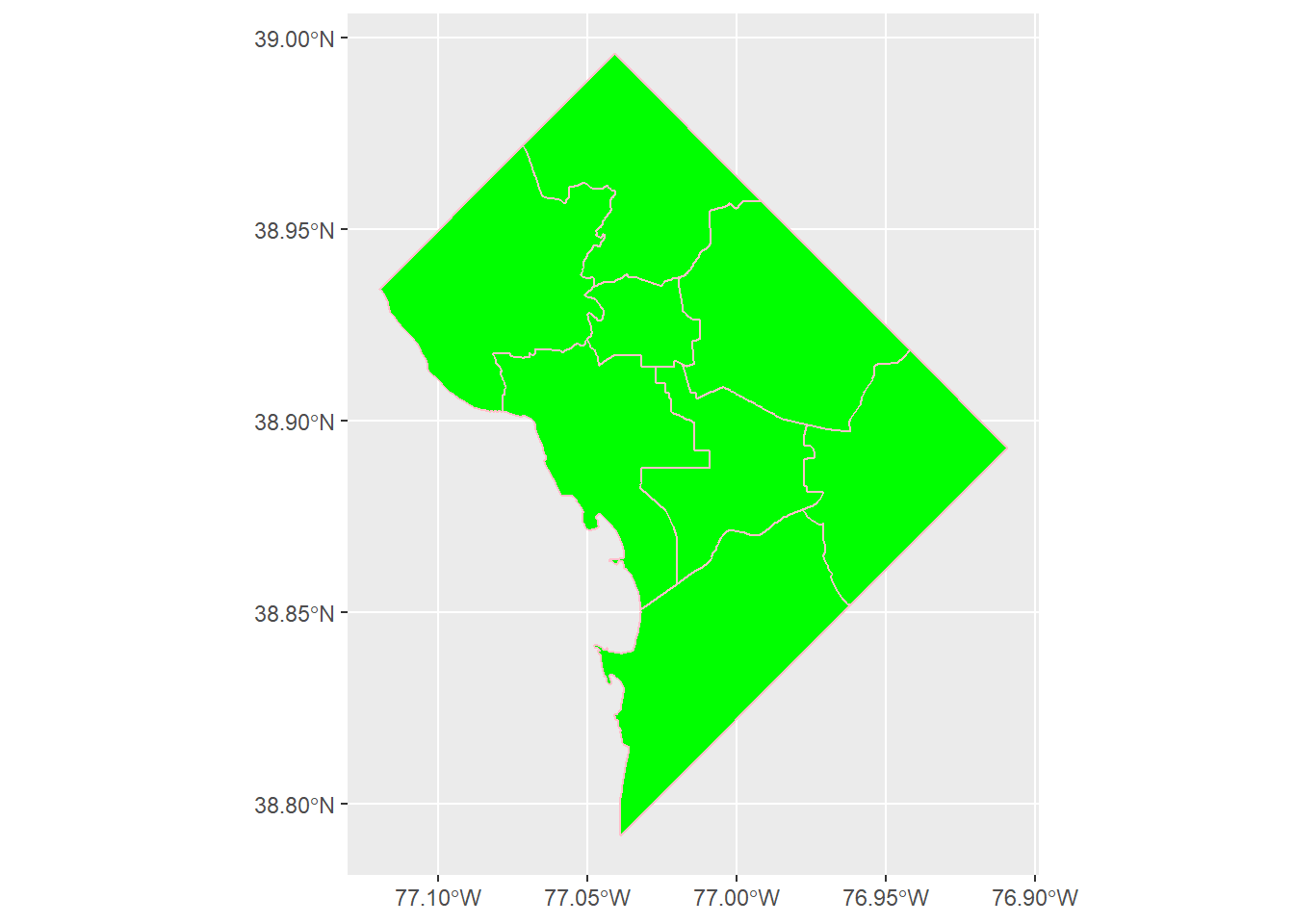
One key function of a map is to identify things. The map above does not identify wards. Let’s fix that. We already have a variable for the ward number, but we have to have a variable that tells R where to put the label. To think about the “where,” remember that a map is sort of like a graph, but where the coordinates are latitude and longitude.
Of course, the current map is polygons, not points. R knows the the locations of the points that bound the polygon, but it doesn’t have the latitude and longitude of the center of the polygon, which is where we’d like to put the label.
Helpfully, there is a built-in R command to do this: geom_sf_text(). This command puts whatever text you specify in label = [variable] at the center of the polygon. (There is also geom_sf_label() if you prefer.)
# plot
ward.map <- ggplot() +
  geom_sf(data = dc.wards) +
  geom_sf_text(data = dc.wards,
               mapping = aes(label=NAME))
ward.map
Warning in st_point_on_surface.sfc(sf::st_zm(x)): st_point_on_surface may not
give correct results for longitude/latitude data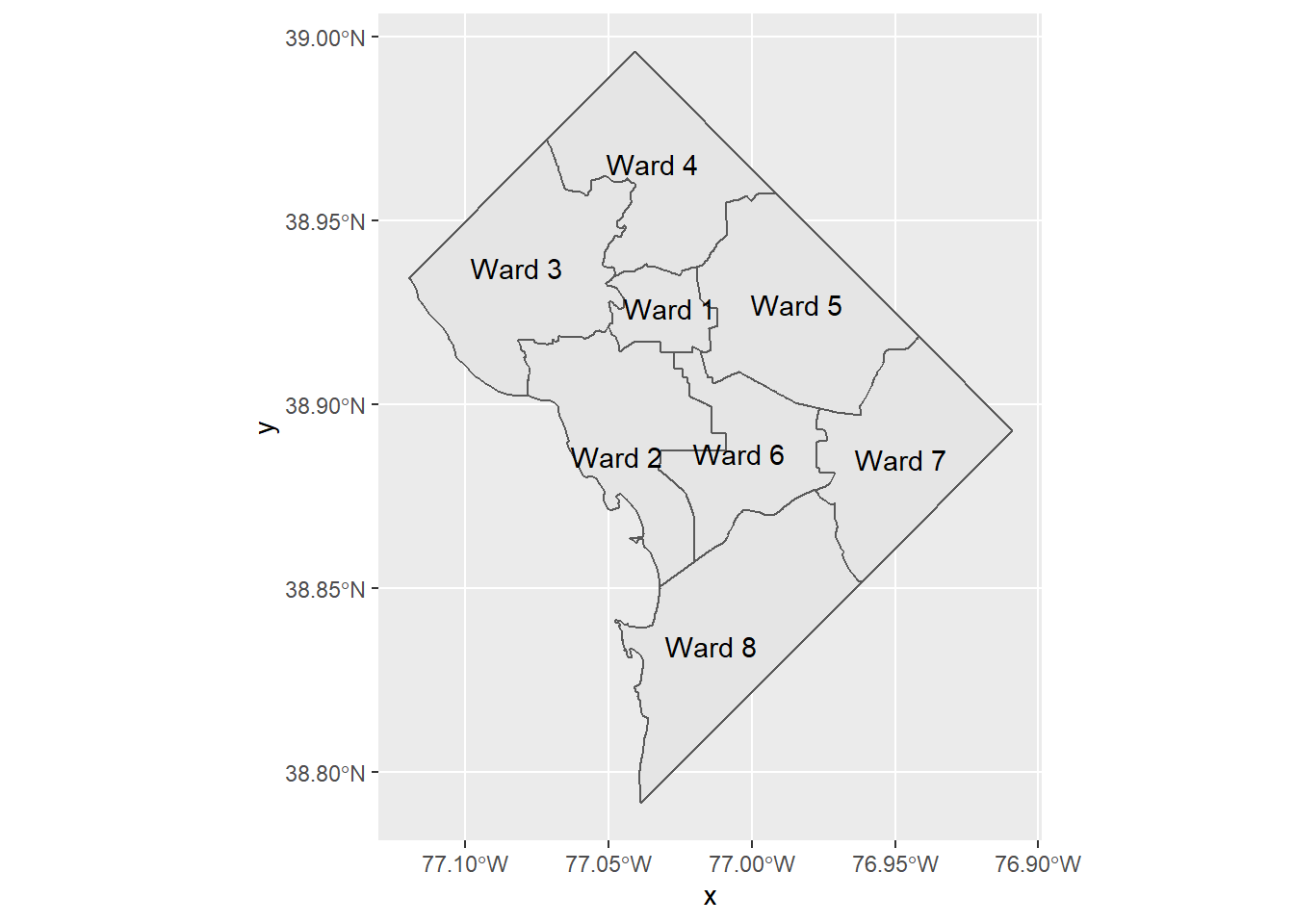
That looks ok, but you might prefer just the ward number, especially if your title makes it clear that these are all wards. You can change what the label says by changing the variable you associate with the label. Below we label by WARD, which is a number for the ward.
# or you can do just the number
ward.map <- ggplot() +
  geom_sf(data = dc.wards) +
  geom_sf_text(data = dc.wards,
                mapping = aes(label=WARD))
ward.map
Warning in st_point_on_surface.sfc(sf::st_zm(x)): st_point_on_surface may not
give correct results for longitude/latitude data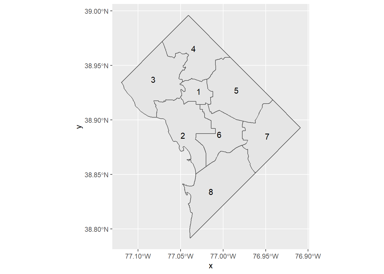
B.4. Plot two things
One of the most powerful things about the combination of sf and ggplot is the ability to plot mutliple features together. To illustrate this, download the location of closed DC public school buildings here. Again, make sure you download the shapefile and save it somewhere you’ll remember. My download was a zipped file that I needed to unzip.
These new data are a points datafile, different from the polygons file we were working with.
Regardless, we load the data, using the same st_read().
# load some points
dcps.pts <- st_read("H:/pppa_data_viz/2022/tutorials/tutorial_05/data/Closed_Public_Schools.shp")
Reading layer `Closed_Public_Schools' from data source
`H:\pppa_data_viz\2022\tutorials\tutorial_05\data\Closed_Public_Schools.shp'
using driver `ESRI Shapefile'
Simple feature collection with 58 features and 37 fields
Geometry type: POINT
Dimension: XY
Bounding box: xmin: -77.06132 ymin: 38.82391 xmax: -76.92087 ymax: 38.96217
Geodetic CRS: WGS 84With these data loaded, add them to the previous map with an additional geom_sf() command, making purple points. Note that you don’t need separate plotting commands for polygons (wards) or points (closed schools).
# plot them
ward.map <- ggplot() +
  geom_sf(data = dc.wards) +
  geom_sf_text(data = dc.wards,
               mapping = aes(label=WARD)) +
  geom_sf(data = dcps.pts,
          color = "purple")
ward.map
Warning in st_point_on_surface.sfc(sf::st_zm(x)): st_point_on_surface may not
give correct results for longitude/latitude data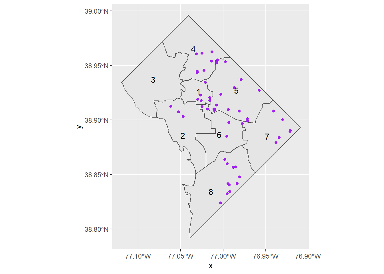
To put two maps on the same chart, they should be in the same projection. R may do this automatically, but you may run into trouble if this fails.
C. Get data from a API
Before working on more map data, we take a detour to learn how to grab data from a Application Programming Interface or API. From our perspective, this is a way to grab data that
- is always updated
- doesn’t require downloading and saving
- can sometimes be customized to particular requests
Basically, a API is a service offered by someone on the Internet. It makes their data available in a standardized format for you to grab.
Here we’re using DC Open Data’s API to grab the same ward map we used in step B.1. above. Start by going to the “about” page for the 2012 ward map. Scroll down to the section on the right that says “I want to…” and open the menu for “View API resources.” Copy the link for the GeoJSON. GeoJSON is a standardized format for shapefiles.
To get this file via API, we need to tell R the API location of the data, as in the first command below. This first command is just defining a variable called map.loc – it’s not doing any processing.
In the next step, we open the file at the address defined by map.loc using the geojson_sf() function. This function – for which we loaded the package geojsonsf at the beginning of the tutorial – grabs the data from the map.loc address in geojson format and creates a simple feature.
# make a variable that says where api data are
map.loc <- "https://opendata.arcgis.com/datasets/0ef47379cbae44e88267c01eaec2ff6e_31.geojson"

# convert from the format the map comes in (geojson) to simple features
map.sf <- geojson_sf(map.loc)

# check
str(map.sf)
Classes 'sf' and 'data.frame': 8 obs. of 86 variables:
$ PCT_BELOW_POV_NAT_AMER : chr "13.9" "54.1" "6" "0" ...
$ NOT_HISPANIC_OR_LATINO : chr "79000" "79843" "66565" "74944" ...
$ PCT_NONFAMILY_HH : chr "62.3192019950125" "39.7794367153037" "42.0445987098464" "57.5190503343528" ...
$ FAMILY_HH : chr "15110" "17747" "17699" "16390" ...
$ TOTAL_HH : chr "40100" "29470" "30539" "38582" ...
$ WARD_ID : chr "6" "8" "4" "3" ...
$ UNEMPLOYMENT_RATE : chr "6.3" "22.9" "9.9" "3.7" ...
$ AGE_85_PLUS : chr "958" "432" "2407" "1837" ...
$ AGE_70_74 : chr "2167" "1904" "2296" "3343" ...
$ PCT_BELOW_POV : chr "12.5" "37.7" "11.9" "9.4" ...
$ PCT_BELOW_POV_WHITE : chr "4.5" "10.8" "5.2" "7.6" ...
$ AGE_65_66 : chr "1518" "1011" "1513" "1574" ...
$ REP_PHONE : chr "(202) 724-8072" "(202) 724-8045" "(202) 724-8052" "(202) 724-8062" ...
$ PCT_BELOW_POV_BLACK : chr "25.7" "38.8" "14.6" "21.7" ...
$ PCT_BELOW_POV_HISP : chr "6.3" "36.3" "14.4" "13.7" ...
$ AGE_55_59 : chr "4724" "5001" "5783" "4388" ...
$ AGE_50_54 : chr "4350" "4978" "6003" "5201" ...
$ AGE_35_39 : chr "8052" "4617" "5913" "6069" ...
$ AGE_80_84 : chr "816" "634" "1753" "1349" ...
$ PCT_BELOW_POV_OTHER : chr "10.7" "51.2" "14.9" "27.1" ...
$ AGE_75_79 : chr "1522" "1026" "2063" "2545" ...
$ CREATED : chr NA NA NA NA ...
$ AGE_30_34 : chr "12512" "5951" "7149" "7374" ...
$ PCT_BELOW_POV_FAM : chr "9.6" "35.3" "8.7" "1.9" ...
$ LABEL : chr "Ward 6" "Ward 8" "Ward 4" "Ward 3" ...
$ AGE_25_29 : chr "13427" "6306" "7039" "8672" ...
$ AGE_22_24 : chr "4596" "4070" "2893" "3849" ...
$ MEDIAN_AGE : chr "33.9" "29.3" "39.3" "37" ...
$ AGE_21 : chr "724" "1748" "668" "1499" ...
$ BACH_DEGREE_25_PLUS : chr "19588" "3781" "13032" "19166" ...
$ AGE_20 : chr "794" "1800" "668" "1497" ...
$ REP_OFFICE : chr "1350 Pennsylvania Ave, Suite 406, NW 20004" "1350 Pennsylvania Ave, Suite 400, NW 20004" "1350 Pennsylvania Ave, Suite 105, NW 20004" "1350 Pennsylvania Ave, Suite 108, NW 20004" ...
$ PCT_BELOW_POV_ASIAN : chr "11.6" "21.6" "10.3" "13.2" ...
$ AGE_67_69 : chr "1596" "1211" "1859" "2602" ...
$ POP_BLACK : chr "29909" "75259" "46884" "5730" ...
$ EDITOR : chr NA NA NA NA ...
$ AGE_60_61 : chr "1830" "1578" "2078" "1992" ...
$ AREASQMI : num 6.22 11.94 9 10.93 10.39 ...
$ REP_EMAIL : chr "callen@dccouncil.us" "twhite@dccouncil.us" "jlewisgeorge@dccouncil.us" "mcheh@dccouncil.us" ...
$ PCT_FAMILY_HH : chr "37.6807980049875" "60.2205632846963" "57.9554012901536" "42.4809496656472" ...
$ MARRIED_COUPLE_FAMILY : chr NA NA NA NA ...
$ AGE_40_44 : chr "5474" "4873" "5760" "5496" ...
$ POP_2000 : num 70867 74049 75179 75335 71440 ...
$ TWO_OR_MORE_RACES : chr "2529" "872" "2287" "3345" ...
$ POP_FEMALE : chr "43879" "45560" "42717" "46001" ...
$ NO_DIPLOMA_25_PLUS : chr "3128" "5958" "3920" "740" ...
$ POP_2010 : num 76238 73662 75773 78887 74308 ...
$ NAME : chr "Ward 6" "Ward 8" "Ward 4" "Ward 3" ...
$ WARD : num 6 8 4 3 5 1 2 7
$ WEB_URL : chr "https://www.dccouncil.us/council/councilmember-allen/" "https://www.dccouncil.us/council/councilmember-trayon-white-sr/" "https://dccouncil.us/council/ward-4-councilmember-janeese-lewis-george/" "https://www.dccouncil.us/council/council-member-mary-m-cheh/" ...
$ POP_25_PLUS_GRADUATE : chr "25882" "2614" "15399" "32503" ...
$ OBJECTID : num 1 2 3 4 5 6 7 8
$ POP_NATIVE_AMERICAN : chr "295" "110" "519" "163" ...
$ POP_ASIAN : chr "3573" "310" "1755" "5188" ...
$ POP_HAWAIIAN : chr "40" "12" "31" "0" ...
$ REP_NAME : chr "Charles Allen" "Trayon White, Sr." "Janeese Lewis George" "Mary M. Cheh" ...
$ POP_OTHER_RACE : chr "1233" "711" "9627" "1864" ...
$ AGE_15_17 : chr "1088" "3596" "2467" "1588" ...
$ POP_MALE : chr "40411" "35573" "40349" "37151" ...
$ AGE_0_5 : chr "4779" "7879" "5602" "4259" ...
$ AGE_10_14 : chr "2235" "5963" "4210" "2814" ...
$ AGE_18_19 : chr "1370" "2945" "1379" "3526" ...
$ NONFAMILY_HH : chr "24990" "11723" "12840" "22192" ...
$ PER_CAPITA_INCOME : chr "58354" "17596" "43880" "83452" ...
$ AGE_45_49 : chr "4524" "4429" "6406" "5025" ...
$ HISPANIC_OR_LATINO : chr "5290" "1290" "16501" "8208" ...
$ AGE_5_9 : chr "2747" "7061" "4421" "4077" ...
$ POP_2011_2015 : num 84290 81133 83066 83152 82049 ...
$ GLOBALID : chr "{5D2A5470-9BA3-4C94-9A21-46B5DBFF70D4}" "{47803E60-D3B3-4445-A139-9456F9B20BED}" "{C0E0D035-7F66-4819-887B-1575851278F3}" "{E6E33839-8446-458B-B7E9-BE071089193C}" ...
$ EDITED : chr NA NA NA NA ...
$ PCT_BELOW_POV_HAWAIIAN : chr "0" "0" "29" "0" ...
$ PCT_BELOW_POV_TWO_RACES : chr "6.2" "36.4" "11.3" "9.8" ...
$ MEDIAN_HH_INCOME : chr "94343" "30910" "74600" "112873" ...
$ NO_DEGREE_25_PLUS : chr "6643" "10975" "10500" "3808" ...
$ POP_25_PLUS : chr NA NA NA NA ...
$ POP_25_PLUS_9TH_GRADE : chr "1785" "1858" "3927" "684" ...
$ MALE_HH_NO_WIFE : chr "944" "1886" "1591" "740" ...
$ FEMALE_HH_NO_HUSBAND : chr "4157" "11653" "5419" "1511" ...
$ PCT_BELOW_POV_WHTE_NOHISP: chr "4.5" "10.8" "5.2" "7.6" ...
$ DIPLOMA_25_PLUS : chr "7079" "18736" "11907" "2139" ...
$ ASSOC_DEGREE_25_PLUS : chr "1852" "2149" "2073" "1003" ...
$ MED_VAL_OOU : chr "573200" "229900" "491300" "823800" ...
$ CREATOR : chr NA NA NA NA ...
$ SHAPEAREA : num 0 0 0 0 0 0 0 0
$ SHAPELEN : num 0 0 0 0 0 0 0 0
$ geometry :sfc_POLYGON of length 8; first list element: List of 1
..$ : num [1:1000, 1:2] -77 -77 -77 -77 -77 ...
..- attr(*, "class")= chr [1:3] "XY" "POLYGON" "sfg"
- attr(*, "sf_column")= chr "geometry"We check the data at the end using the head() command and see a simple feature file with eight wards.
Using a API helps us skip a downloading step. But in addition, if we were repeating this task every month, this would also grab the updated file.
APIs can also be customized to ask for specific data. The Census Bureau, for example, lets you make a API call specific to a dataset, jurisdiction, and variable. So you could set up a call to ask for the income in a specific state and year, or a set of states and years.
D. Use bigger data
Now we are going to use a larger dataset and try to make a presentation-quality map.
D.1. Load crime data
For this portion of the tutorial, we’ll use DC crime data. Download 2018 DC crime data as a shapefile from here; then use st_read() to read in the file. (Alternatively, you can try the API trick you just learned in step C.)
# load data
c2018 <- st_read("H:/pppa_data_viz/2019/tutorial_data/lecture05/Crime_Incidents_in_2018/Crime_Incidents_in_2018.shp")
Reading layer `Crime_Incidents_in_2018' from data source
`H:\pppa_data_viz\2019\tutorial_data\lecture05\Crime_Incidents_in_2018\Crime_Incidents_in_2018.shp'
using driver `ESRI Shapefile'
Simple feature collection with 33645 features and 23 fields
Geometry type: POINT
Dimension: XY
Bounding box: xmin: -77.11232 ymin: 38.81467 xmax: -76.91002 ymax: 38.9937
Geodetic CRS: WGS 84Each row in this dataframe is a crime, with attendant information, including the specific location of the crime.
It is always a good idea to do some quick checks on data quality. The note on DC Open data’s page about missing values made me nervous, but using summary() to look at the geographic information suggests it is ok.
First we look at the variable definitions:
# look at variables
str(c2018)
Classes 'sf' and 'data.frame': 33645 obs. of 24 variables:
$ CCN : chr "07006630" "10954295" "12146972" "17070029" ...
$ REPORT_DAT: chr "2018-07-26T00:00:00.000Z" "2018-04-05T21:17:59.000Z" "2018-07-31T00:00:00.000Z" "2018-01-09T00:00:00.000Z" ...
$ SHIFT : chr "MIDNIGHT" "EVENING" "MIDNIGHT" "MIDNIGHT" ...
$ METHOD : chr "GUN" "OTHERS" "OTHERS" "GUN" ...
$ OFFENSE : chr "HOMICIDE" "SEX ABUSE" "HOMICIDE" "HOMICIDE" ...
$ BLOCK : chr "3100 3198 BLOCK OF 24TH STREET SE" "3810 - 3899 BLOCK OF RESERVOIR ROAD NW" "1700 - 1799 BLOCK OF BENNING ROAD NE" "2600 - 2631 BLOCK OF MARTIN LUTHER KING JR AVENUE SE" ...
$ XBLOCK : num 402412 393499 401872 400393 400863 ...
$ YBLOCK : num 131645 138307 136822 132326 132294 ...
$ WARD : chr "8" "2" "6" "8" ...
$ ANC : chr "8B" "2E" "6A" "8C" ...
$ DISTRICT : chr "7" "2" "5" "7" ...
$ PSA : chr "702" "206" "507" "703" ...
$ NEIGHBORHO: chr "Cluster 36" "Cluster 4" "Cluster 23" "Cluster 37" ...
$ BLOCK_GROU: chr "007408 1" "000201 1" "007901 1" "007401 2" ...
$ CENSUS_TRA: chr "007408" "000201" "007901" "007401" ...
$ VOTING_PRE: chr "Precinct 115" "Precinct 6" "Precinct 81" "Precinct 119" ...
$ LATITUDE : num 38.9 38.9 38.9 38.9 38.9 ...
$ LONGITUDE : num -77 -77.1 -77 -77 -77 ...
$ BID : chr NA NA NA "ANACOSTIA" ...
$ START_DATE: chr "2007-01-14T23:30:00.000Z" "2018-04-01T00:01:17.000Z" "2012-10-18T00:10:00.000Z" "2017-04-28T12:21:45.000Z" ...
$ END_DATE : chr "2007-01-14T00:00:00.000Z" "2018-04-05T21:18:34.000Z" "2012-10-18T00:12:00.000Z" NA ...
$ OBJECTID : num 2.59e+08 2.59e+08 2.59e+08 2.59e+08 2.59e+08 ...
$ OCTO_RECOR: chr "07006630-01" "10954295-01" "12146972-01" "17070029-01" ...
$ geometry :sfc_POINT of length 33645; first list element: 'XY' num -77 38.9
- attr(*, "sf_column")= chr "geometry"
- attr(*, "agr")= Factor w/ 3 levels "constant","aggregate",..: NA NA NA NA NA NA NA NA NA NA ...
..- attr(*, "names")= chr [1:23] "CCN" "REPORT_DAT" "SHIFT" "METHOD" ...Then I check out a few specific variables. In reviewing the tutorial, one year’s TA found different values for this summary – so don’t worry if yours do not match mine exactly.
# size and missings
dim(c2018)
[1] 33645 24summary(c2018$LATITUDE) Min. 1st Qu. Median Mean 3rd Qu. Max.
38.81 38.89 38.91 38.91 38.92 38.99 summary(c2018$LONGITUDE) Min. 1st Qu. Median Mean 3rd Qu. Max.
-77.11 -77.03 -77.01 -77.01 -76.99 -76.91 table(c2018$OFFENSE, useNA = "always")
                     ARSON ASSAULT W/DANGEROUS WEAPON
                         5                       1668
                  BURGLARY                   HOMICIDE
                      1415                        160
       MOTOR VEHICLE THEFT                    ROBBERY
                      2388                       2019
                 SEX ABUSE               THEFT F/AUTO
                       275                      11574
               THEFT/OTHER                       <NA>
                     14141                          0
There does not seem to be an overwhelming number of missing values (NAs).
D.2. Making legible maps from these data
There are so many crimes in these data that a picture that maps them all is not a good idea. So we make a marker for the violent crimes (arson, assault, homicide, robbery and sex abuse) only. We use a ifelse() command to discriminate between the two types. After creating the new variable ctype, I use the table() command to check whether I’ve put the right crimes in each group.
Note that I use some shorthand code so I don’t have to write six equalities. Writing c2018$OFFENSE %in% c("ARSON","ASSAULT W/DANGEROUS WEAPON") is equivalent to writing c2018$OFFENSE == "ARSON" | c2018$OFFENSE == "ASSAULT W/DANGEROUS WEAPON". The first is shorter and easier to debug.
# wrong!
c2018$ctype <- ifelse(test = c2018$OFFENSE %in% c("ARSON","ASSAULT  W/DANGEROUS WEAPON",
                                                  "HOMICIDE", "ROBBERY", "SEX ABUSE"),
                      yes = 1,
                      no = 0)
It is always a good idea to check your work. As we see below, using a check with the table() command, my coding did not catching all violent crimes.
table(c2018$ctype, c2018$OFFENSE)
    ARSON ASSAULT W/DANGEROUS WEAPON BURGLARY HOMICIDE MOTOR VEHICLE THEFT
  0     0                       1668     1415        0                2388
  1     5                          0        0      160                   0

    ROBBERY SEX ABUSE THEFT F/AUTO THEFT/OTHER
  0       0         0        11574       14141
  1    2019       275            0           0
The “assault with a dangerous weapon” should have been a violent crime, but it is not An extra space above that caused trouble. I fix and try again:
# better!
c2018$ctype <- ifelse(test = c2018$OFFENSE %in% c("ARSON","ASSAULT W/DANGEROUS WEAPON",
                                                  "HOMICIDE", "ROBBERY", "SEX ABUSE"),
                      yes = 1,
                      no = 0)
table(c2018$ctype, c2018$OFFENSE)
    ARSON ASSAULT W/DANGEROUS WEAPON BURGLARY HOMICIDE MOTOR VEHICLE THEFT
  0     0                          0     1415        0                2388
  1     5                       1668        0      160                   0

    ROBBERY SEX ABUSE THEFT F/AUTO THEFT/OTHER
  0       0         0        11574       14141
  1    2019       275            0           0
Now this looks ok. All crimes that I listed as violent show up as having c2018$ctype == 1.
Another way to check the data is to plot them. Do this below. But if your computer chokes, just ignore this step:
# plot
crimeo <- ggplot() +
  geom_sf(data = c2018, aes(fill = ctype))
crimeo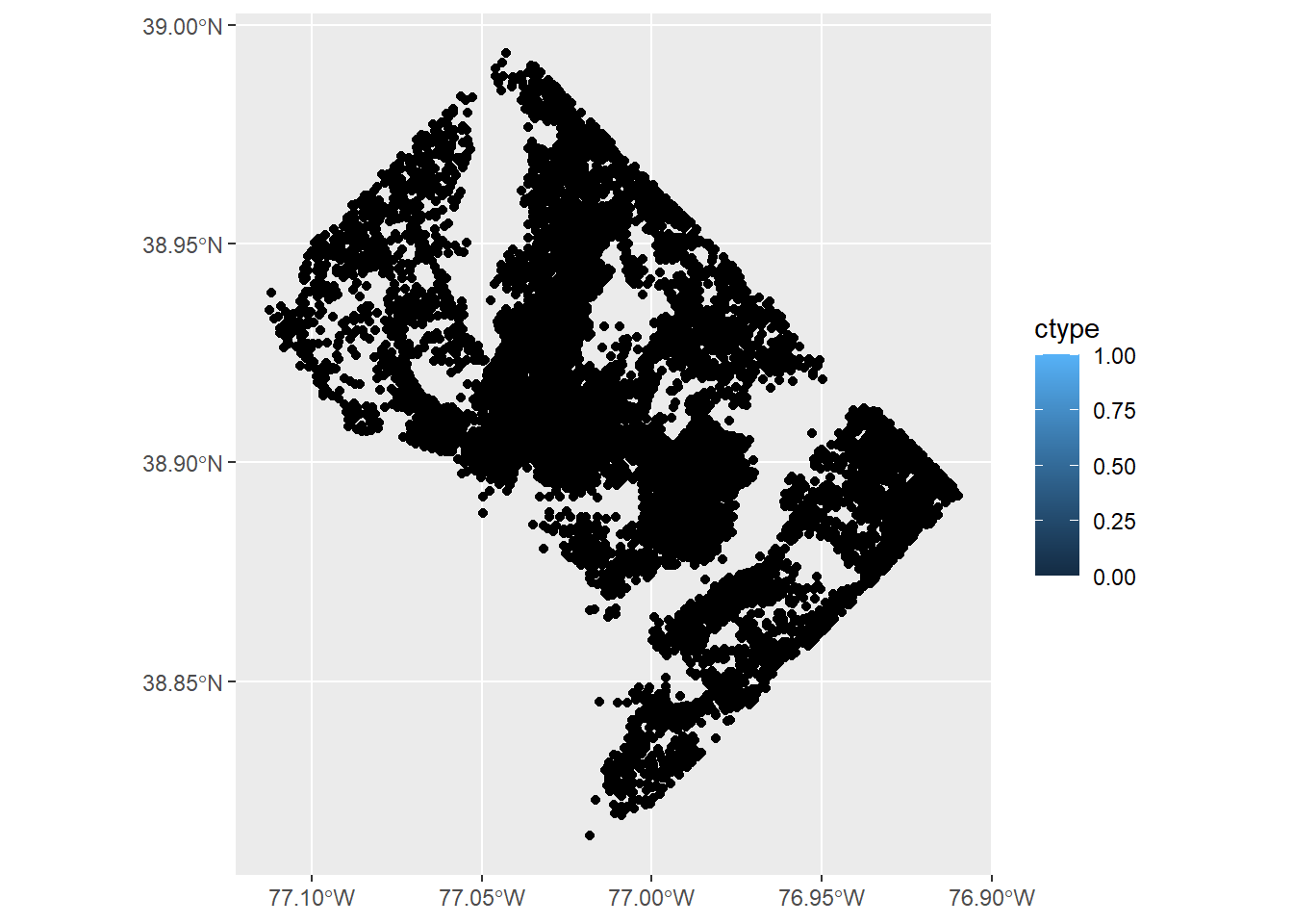
This is so many points that it’s hard to make sense of the map.
One way to have a map that is legible is to focus on crimes with fewer occurences. To this end, we subset to a smaller dataframe with just homicides and burglaries. We use the type of subsetting we’ve already learned. Recall that the statement (c2018$OFFENSE == "HOMICIDE" | c2018$OFFENSE == "BURGLARY") is true if the offense is either a homicide or a burglary. The | operator means “or” (in R and many other languages).
# make smaller dataframe
vc2018 <- c2018[which(c2018$OFFENSE == "HOMICIDE" | c2018$OFFENSE == "BURGLARY"),]
The vc2018 dataframe should have fewer observations than c2018 – you can check that it does with dim().
Now let’s plot homicides and burglaries. The code is similar to before, but relies on different data. Notice the change in the data = input. Analogous to what we do with bar graphs, we use fill for the offense. Notice that this is inside the aes() command.
# lets just do homicides and burglary -- bad
vc <- ggplot() +
  geom_sf(data = vc2018,
          mapping = aes(fill = OFFENSE))
vc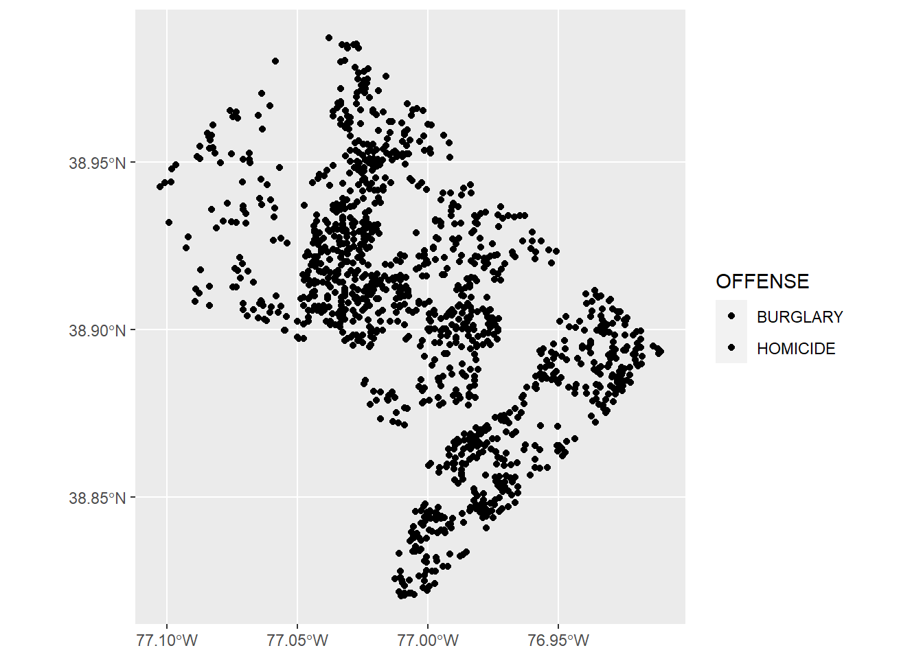
This was not a good idea! From the legend, R knows that we’re trying to use these two types, but there’s nothing to see in the plot. Rather than fill=, use color=. Color is for lines and dots. Fill is for bars and other shapes.
# lets just do homicides and burglary -- better
vc <- ggplot() +
  geom_sf(data = vc2018,
          mapping = aes(color = OFFENSE))
vc
But the legend now looks a little wacky. Use both color and fill to get something reasonable looking.
# lets just do homicides and burglary -- best
vc <- ggplot() +
  geom_sf(data = vc2018,
          mapping = aes(color = OFFENSE, fill = OFFENSE))
vc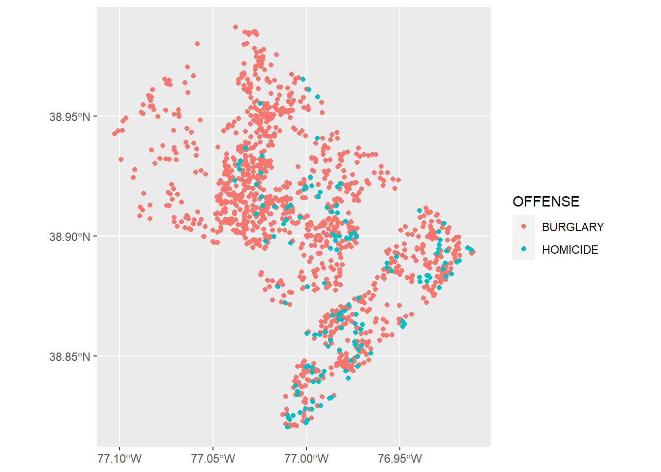
Of course, this map still looks ugly. I very much like the map here, made entirely in ggplot and sf.
To clean up this map, I’ve mostly copied Timo’s work, particularly the theme elements of the map. See the next command below.
I’d like to also add ward boundaries to the map. Here is a first attempt.
# make it look decent -- but wrong layer on top!
vc <- ggplot() +
  geom_sf(data = vc2018,
          mapping = aes(color = OFFENSE, fill = OFFENSE)) +
  geom_sf(data = dc.wards) +
  theme(
    text = element_text(color = "#22211d"),
    axis.line = element_blank(),
    axis.text.x = element_blank(),
    axis.text.y = element_blank(),
    axis.ticks = element_blank(),
    axis.title.x = element_blank(),
    axis.title.y = element_blank(),
    panel.grid.major = element_blank(),
    panel.grid.minor = element_blank(),
    plot.background = element_rect(fill = "#f5f5f2", color = NA),
    panel.background = element_rect(fill = "#f5f5f2", color = NA),
    legend.background = element_rect(fill = "#f5f5f2", color = NA)
    )
vc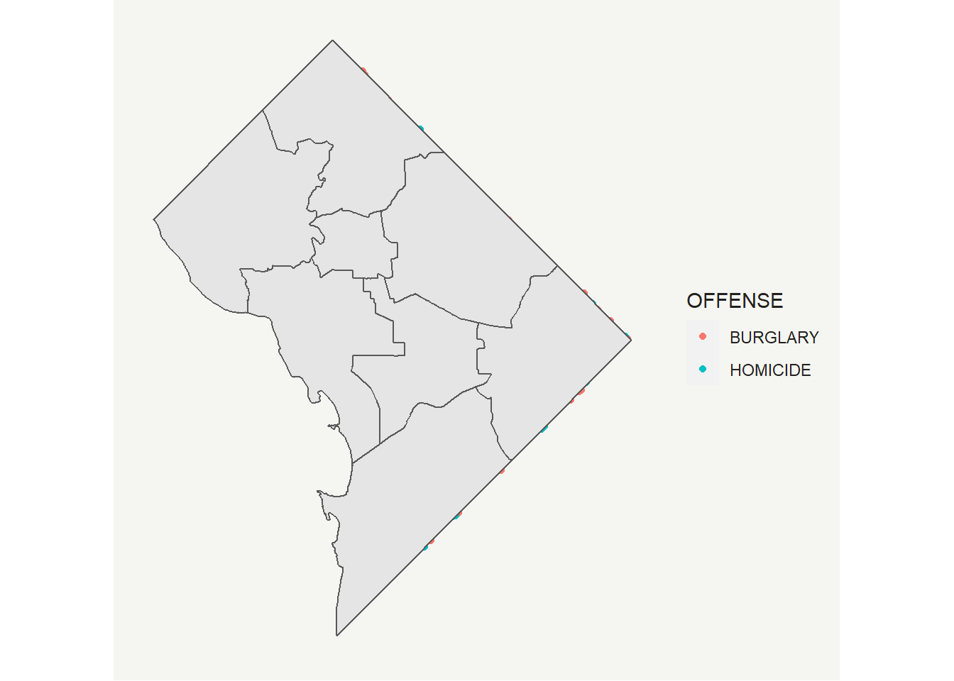
This looks bad! The code above does not give a good result because the wards are on top of the points. Note that R draws the maps in the order you call them, so that the last one is on top.
We can fix this ordering issue by switching the order of the layering. By putting the wards first in the command, they go first on the map. Then points (vc2018) on top.
# make it look decent -- fixed layer issue
# subsantially copied from
# https://timogrossenbacher.ch/2016/12/beautiful-thematic-maps-with-ggplot2-only/
vc <- ggplot() +
  geom_sf(data = dc.wards, color = "white", fill = "grey") +
  geom_sf(data = vc2018, aes(color = OFFENSE, fill = OFFENSE)) +
  theme(
    text = element_text(color = "#22211d"),
    axis.line = element_blank(),
    axis.text.x = element_blank(),
    axis.text.y = element_blank(),
    axis.ticks = element_blank(),
    axis.title.x = element_blank(),
    axis.title.y = element_blank(),
    plot.background = element_rect(fill = "#f5f5f2", color = NA),
    panel.background = element_rect(fill = "#f5f5f2", color = NA),
    panel.grid = element_line(color = "#f5f5f2"),
    legend.background = element_rect(fill = "#f5f5f2", color = NA),
    legend.position = c(0.13,0.2)
  )
vc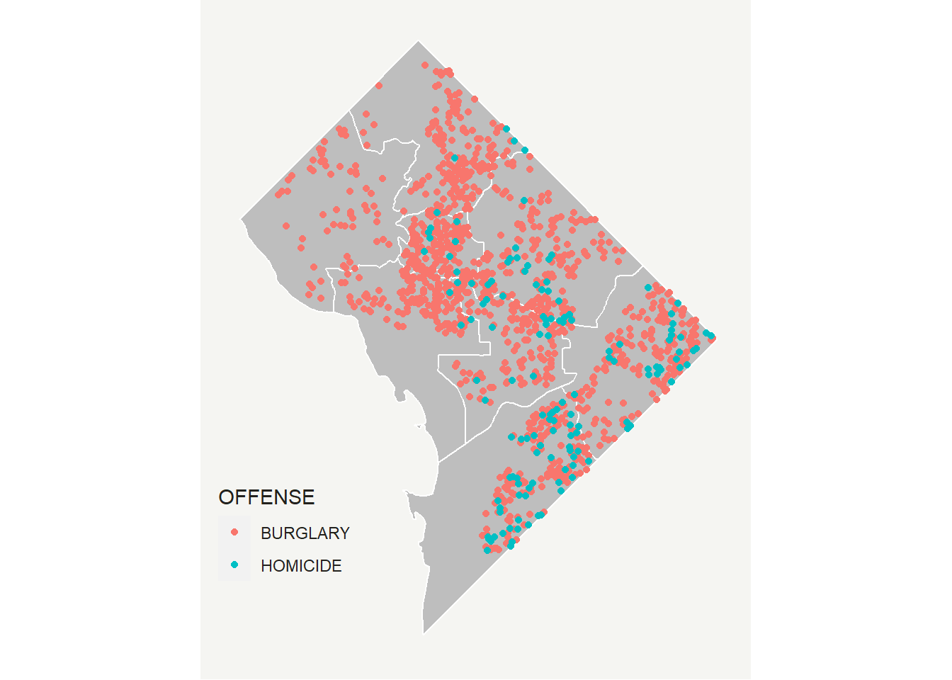
Now save this file using ggsave() as we learned in Tutorial 4.
Before doing that, I make a variable (or a 1x1 matrix, if you prefer) that has today’s date in it, in numeric form (e.g., 20230218). I like to always put the date in the name of anything I save so that when I work on it again I will not save over the older version.
R has a built in function to deliver today’s date (Sys.Date()). I use the substring command (see lecture 4 notes) to extract the parts we need. I then use paste0 to put the parts together. This command puts together all the text bits you put into it, with no spaces in between (the 0 part). You can look at all the parts separately if you’d like to better understand what’s going on.
# save using ggsave
# todays date
Sys.Date()
[1] "2023-04-24"dateo <- paste0(substr(Sys.Date(),1,4),
substr(Sys.Date(),6,7),
substr(Sys.Date(),9,10))
dateo[1] "20230424"Now with this date in hand, I make the filename with the date in it. If you don’t specific the full file path, R saves your file in the “current working directory.” The current working directory may not the directory your program is in. (You can see what directory you’re in with the getwd() command).
The ggsave() code has one modification from Tutorial 4. Before the ggsave() command, I create a variable that has the filename for the file I’d like to save. Sometimes this makes the programming clearer. So, instead of the long filename in the filename = portion of the ggsave, I put the variable (patho) that I just created.
fn <- paste0(dateo,"_violent_crime_2018.jpg")
patho <- paste0("H:/pppa_data_viz/2020/tutorials/tutorial_05/",fn)
ggsave(filename = patho,
       plot = vc,
       device = "jpg",
       dpi = 300)
Saving 7 x 5 in imageE. Putting map data together with other data
Part of the value data in a spatial format is your ability to combine data spatially. This means you can combine data not just by merging variables, but by saying “what polygon does this point fall in?” or “which polygons does this polygon touch?”
We now perform such a spatial analysis. For our example, we’ll use the crime data and find the block group in which each crime takes place.
This could be useful for a number of reasons. For example, suppose you want to know if poor neighoborhoods have more crimes, or if neighborhoods with more shade trees have more crimes. For either of these questions, you need to know infomation by neighborhoods.
How do you go from what you have now to that? Right now, you have a dataframe at the level of the individual crime. To ask questions about neighborhoods, you need neighborhood level data.
In this tutorial, we will use neighborhood information to compute crime rates: total neighborhood crimes divided by neighborhood population. We already have crimes, but we have to associate each crime with an area, and we need to know the population of each of these areas.
To give an overview, we need to
- find the block group (neighborhood) in which each crime is located
- find the total number of crimes in each block group by type \(\rightarrow\) block group level data
- merge in other block group information, including population
- calculate a rate
E.1. Find the block group of each point
We begin by loading the block group map from the DC open data website; be sure to download the shapefile.
Load the block group data – note that it is a shapefile so we use st_read() and see what variables it has.
# load block group map
bg2010 <- st_read("H:/pppa_data_viz/2019/tutorial_data/lecture05/Census_Block_Groups__2010/Census_Block_Groups__2010.shp")
Reading layer `Census_Block_Groups__2010' from data source
`H:\pppa_data_viz\2019\tutorial_data\lecture05\Census_Block_Groups__2010\Census_Block_Groups__2010.shp'
using driver `ESRI Shapefile'
Simple feature collection with 450 features and 54 fields
Geometry type: POLYGON
Dimension: XY
Bounding box: xmin: -77.11976 ymin: 38.79165 xmax: -76.9094 ymax: 38.99581
Geodetic CRS: WGS 84names(bg2010) [1] "OBJECTID" "TRACT" "BLKGRP" "GEOID" "P0010001"
[6] "P0010002" "P0010003" "P0010004" "P0010005" "P0010006"
[11] "P0010007" "P0010008" "OP000001" "OP000002" "OP000003"
[16] "OP000004" "P0020002" "P0020005" "P0020006" "P0020007"
[21] "P0020008" "P0020009" "P0020010" "OP00005" "OP00006"
[26] "OP00007" "OP00008" "P0030001" "P0030003" "P0030004"
[31] "P0030005" "P0030006" "P0030007" "P0030008" "OP00009"
[36] "OP00010" "OP00011" "OP00012" "P0040002" "P0040005"
[41] "P0040006" "P0040007" "P0040008" "P0040009" "P0040010"
[46] "OP000013" "OP000014" "OP000015" "OP000016" "H0010001"
[51] "H0010002" "H0010003" "SHAPE_Leng" "SHAPE_Area" "geometry" Let’s plot it on the same map as the crime points to make sure that the maps are what we think they are.
# look at it with homicides and burglaries
cbg <- ggplot() +
  geom_sf(data = bg2010, color = "white", fill = "grey") +
  geom_sf(data = vc2018, aes(color = OFFENSE, fill = OFFENSE)) +
  theme(
    text = element_text(color = "#22211d"),
    axis.line = element_blank(),
    axis.text.x = element_blank(),
    axis.text.y = element_blank(),
    axis.ticks = element_blank(),
    axis.title.x = element_blank(),
    axis.title.y = element_blank(),
    plot.background = element_rect(fill = "#f5f5f2", color = NA),
    panel.background = element_rect(fill = "#f5f5f2", color = NA),
    panel.grid = element_blank(),
    legend.background = element_rect(fill = "#f5f5f2", color = NA),
    legend.position = c(0.13,0.2)
  )
cbg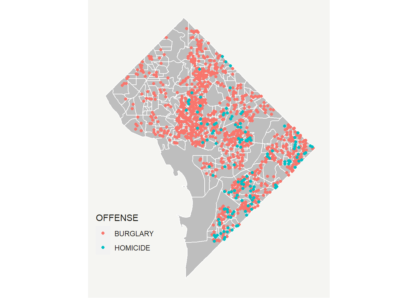
This quick look suggests that all crimes are inside a block group. Now we need to find which block group. To do this, we use a command called st_intersection(). When the shapefiles are points and polygons (in that order) as in the call below, R returns a points dataframe with information on the block group into which each point falls.
If this seems confusing, please go back to the lecture notes and look at the example about this type of intersection.
Let’a also make the intersection easier on ourselves by making a smaller version of the block group data (bg2010.small) that has just the block group id variables – that’s all we want to add to the points and it is helpful to reduce the number of variables we need to keep track of.
# find which crimes are in which block groups
bg2010.small <- bg2010[,c("TRACT","BLKGRP")]
dim(bg2010.small)
[1] 450 3Finally, before intersecting, make sure both simple features have the same projection. If the files do not, the intersection will either fail or give you garbage.
st_crs(vc2018)Coordinate Reference System:
User input: WGS 84
wkt:
GEOGCRS["WGS 84",
DATUM["World Geodetic System 1984",
ELLIPSOID["WGS 84",6378137,298.257223563,
LENGTHUNIT["metre",1]]],
PRIMEM["Greenwich",0,
ANGLEUNIT["degree",0.0174532925199433]],
CS[ellipsoidal,2],
AXIS["latitude",north,
ORDER[1],
ANGLEUNIT["degree",0.0174532925199433]],
AXIS["longitude",east,
ORDER[2],
ANGLEUNIT["degree",0.0174532925199433]],
ID["EPSG",4326]]st_crs(bg2010.small)Coordinate Reference System:
User input: WGS 84
wkt:
GEOGCRS["WGS 84",
DATUM["World Geodetic System 1984",
ELLIPSOID["WGS 84",6378137,298.257223563,
LENGTHUNIT["metre",1]]],
PRIMEM["Greenwich",0,
ANGLEUNIT["degree",0.0174532925199433]],
CS[ellipsoidal,2],
AXIS["latitude",north,
ORDER[1],
ANGLEUNIT["degree",0.0174532925199433]],
AXIS["longitude",east,
ORDER[2],
ANGLEUNIT["degree",0.0174532925199433]],
ID["EPSG",4326]]This looks good. But if you want to be clever, you can even test their equality:
proj.test <- "nada"
proj.test <- ifelse(test = (st_crs(vc2018) == st_crs(bg2010.small)),
                    yes = "yes",
                    no = "no")
print(paste0("Are the projections the same? ", proj.test))
[1] "Are the projections the same? yes"Now that we’ve confirmed the two projections are the same, use this smaller dataframe to do the points and polygons intersection:
# find which crimes are in which block groups
cbg <- st_intersection(vc2018,bg2010.small)
Warning: attribute variables are assumed to be spatially constant throughout all
geometriesIt is critically important to check the output.
dim(cbg)[1] 1567 27head(cbg)Simple feature collection with 6 features and 26 fields
Geometry type: POINT
Dimension: XY
Bounding box: xmin: -77.0734 ymin: 38.90259 xmax: -77.05759 ymax: 38.91258
Geodetic CRS: WGS 84
CCN REPORT_DAT SHIFT METHOD OFFENSE
1826 18064713 2018-04-23T13:04:28.000Z DAY OTHERS BURGLARY
11452 18134729 2018-08-14T03:10:42.000Z MIDNIGHT OTHERS BURGLARY
26674 18042061 2018-03-15T16:09:21.000Z EVENING OTHERS BURGLARY
30745 18026424 2018-02-16T14:31:32.000Z DAY OTHERS BURGLARY
30750 18026435 2018-02-16T15:42:03.000Z EVENING OTHERS BURGLARY
23472 18136654 2018-08-17T04:38:28.000Z MIDNIGHT OTHERS BURGLARY
BLOCK XBLOCK YBLOCK WARD ANC
1826 3100 - 3199 BLOCK OF K STREET NW 394626 137194 2 2E
11452 3036 - 3099 BLOCK OF M STREET NW 394737 137483 2 2E
26674 3000 - 3099 BLOCK OF N STREET NW 394778 137665 2 2E
30745 2800 - 2899 BLOCK OF PENNSYLVANIA AVENUE NW 395005 137471 2 2E
30750 2800 - 2899 BLOCK OF PENNSYLVANIA AVENUE NW 395005 137471 2 2E
23472 3700 - 3799 BLOCK OF RESERVOIR ROAD NW 393634 138304 2 2E
DISTRICT PSA NEIGHBORHO BLOCK_GROU CENSUS_TRA VOTING_PRE LATITUDE
1826 2 206 Cluster 4 000100 4 000100 Precinct 5 38.90258
11452 2 206 Cluster 4 000100 4 000100 Precinct 5 38.90519
26674 2 206 Cluster 4 000100 4 000100 Precinct 5 38.90683
30745 2 206 Cluster 4 000100 4 000100 Precinct 5 38.90508
30750 2 206 Cluster 4 000100 4 000100 Precinct 5 38.90508
23472 2 206 Cluster 4 000201 1 000201 Precinct 6 38.91258
LONGITUDE BID START_DATE END_DATE
1826 -77.06195 GEORGETOWN 2018-04-23T10:56:35.000Z <NA>
11452 -77.06068 GEORGETOWN 2018-08-13T22:52:11.000Z 2018-08-14T00:19:42.000Z
26674 -77.06021 <NA> 2018-03-14T03:48:45.000Z 2018-03-14T03:49:12.000Z
30745 -77.05759 GEORGETOWN 2018-02-16T01:25:28.000Z 2018-02-16T02:30:15.000Z
30750 -77.05759 GEORGETOWN 2018-02-15T17:30:53.000Z 2018-02-16T08:15:53.000Z
23472 -77.07340 <NA> 2018-08-17T03:36:29.000Z 2018-08-17T03:46:04.000Z
OBJECTID OCTO_RECOR ctype TRACT BLKGRP geometry
1826 259183436 18064713-01 0 000100 4 POINT (-77.06196 38.90259)
11452 259193062 18134729-01 0 000100 4 POINT (-77.06068 38.9052)
26674 259240847 18042061-01 0 000100 4 POINT (-77.06021 38.90684)
30745 259245997 18026424-01 0 000100 4 POINT (-77.05759 38.90509)
30750 259246002 18026435-01 0 000100 4 POINT (-77.05759 38.90509)
23472 259224604 18136654-01 0 000201 1 POINT (-77.0734 38.91258)This file should have the same number of rows as the crime points datafile. It should have variables from both the crime points file and the block group file. Does this seem right?
Now I can start to find the average number of crimes per person. This is a multi-step process:
- find the block group in which each crime is located (done)
- find the total number of crimes in each block group for each type \(\rightarrow\) block group level data
- merge in the block group population
- calculate a rate
E.2. Total number of crimes per block group
The next step in this process of finding a crime rate by block group is to find the total number of crimes by type in each block group. Remember that the current dataset is at the crime level – one observation per crime. We want a dataset at the block group/offense level – so we know how many offenses of each type are committed in each block group in 2018.
We want R to just count the number of observations by block group and offense. We do this by grouping the data by tract/block group/offense, and then summarizing (counting) the number of observations in each group (n()).
Before any summing up, we make cbg from a simple feature file into a regular dataframe by setting the geometry part of the file to “NULL.” This is always a good idea if you don’t need the geometric features (we don’t here), because maps take a lot more memory and slow things down. Also, in the following step we are going to merge with the block group shapefile, and you cannot merge two shapefiles together (which shape would you take?).
# first count number of crimes by type by block group
dim(cbg)
[1] 1567 27st_geometry(cbg ) <- NULL
cbg <- group_by(.data = cbg, TRACT, BLKGRP, OFFENSE)
cbgs <- summarize(.data = cbg, incidents = n())`summarise()` has grouped output by 'TRACT', 'BLKGRP'. You can override using
the `.groups` argument.This new dataframe should have two rows for each block group, if each block group has both types of crimes (homicides and burglaries). Since not all block groups have homicides (thank goodness), the total number of observations should be less than the total number of block groups times two. Under NO circumstances should it ever be more. So a good first initial check on this dataframe (cbgs) is to see how many rows it has relative to the block group file. It should have more, but never more than twice as much.
# total number of observations and variables in new block group/crime file
dim(cbgs)
[1] 478 4# total number of observations and variables in block group file
dim(bg2010.small)[1] 450 3Things look ok.
Let’s check this work a different way by making a quick histogram of burglaries to see if our numbers seem reasonable (homicides, thankfully, are more rare, so they are less amenable to this kind of check). Note that this shows only block groups with at least one burglary. (We could fix this with what we do later in this step.)
# make a histogram of the distribution of burlargies
burg.hist <- ggplot() +
  geom_histogram(data = cbgs[which(cbgs$OFFENSE == "BURGLARY"),],
                 mapping = aes(x = incidents))
burg.hist
`stat_bin()` using `bins = 30`. Pick better value with `binwidth`.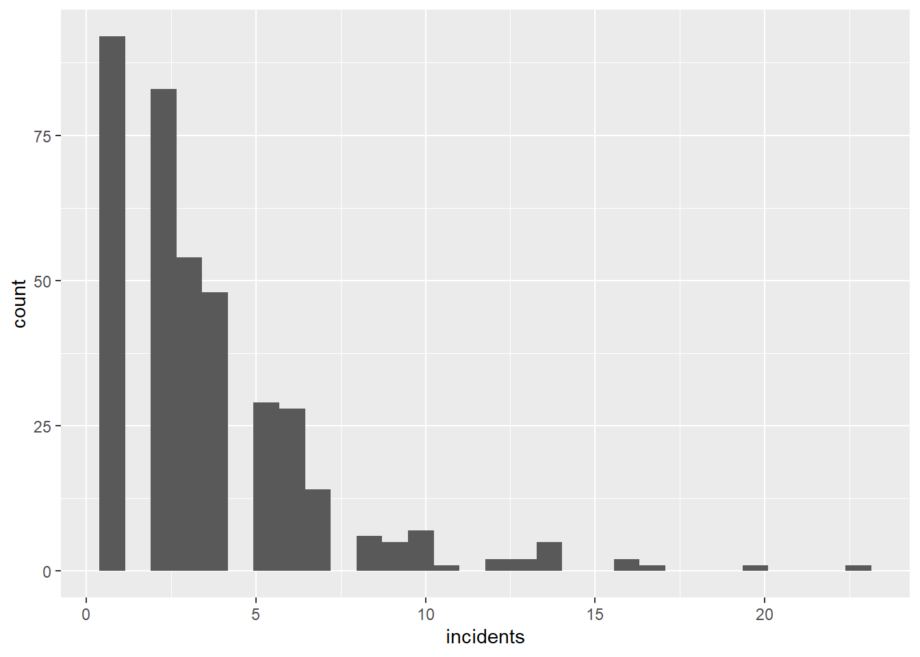
Look at these numbers. Do these seem like plausible numbers for burglaries in a given year in a block group?
So now you have successfully created a block group/offense level dataframe (one row per block group and offense type).
E.3. Add block group population
Now we are ready to undertake the third step, which is mergning in block group population.
Remember, the steps are
- find the block group in which each crime is located (done)
- find the total number of crimes in each block group for each type \(\rightarrow\) block group level data (done)
- merge in block group population
- calculate a rate
We do this because it’s useful to know not just the level of crime, but the crime rate. We find a crime rate by dividing the number of crimes by the resident population (what is the right denominator is a big issue for criminologists; for now we’ll suffice with resident population).
To make a rate, we need the resident population of each block group. I know that the block group shapefile has a population variable. It’s poorly labeled online, but I know from other work that P0010001 is actually total population.
We cannot merge a spatial dataframe (cbgs) and another spatial dataframe (bgs.2010). R would be confused and not know which shapes to use.
# need to merge in block group population
# i know that total population is P0010001
bg2010.pop <- bg2010[,c("TRACT","BLKGRP","P0010001")]
st_geometry(bg2010.pop) <- NULL
Now we have a new dataframe called bg2010.pop that has no spatial information and three variables. Next we merge with dataframe with the cbg dataframe by two variables: tract and block group. (If you were using more than just one state’s worth of data, you would need to include the state ID as well; tract numbers repeat across states.) We specify the by = to have two variables using this c() notation. We use all = TRUE to keep all observations from both dataframes. This has the effect of keeping all block groups, meaning that we have block groups even when they have no homicides or burglaries. This allows us to calculate crime rates of zero.
After this merge (as with any merge), we check the size of the output dataframe relative to the size of the input dataframes.
cbgs2 <- merge(x = cbgs,
               y = bg2010.pop,
               by = c("TRACT","BLKGRP"),
               all.x = TRUE)
print("here is the size of the block group level crime data")
[1] "here is the size of the block group level crime data"dim(cbgs)[1] 478 4print("here is the size of the block group demographic data")[1] "here is the size of the block group demographic data"dim(bg2010.pop)[1] 450 3print("here is the size of the merged dataframe")[1] "here is the size of the merged dataframe"dim(cbgs2) [1] 478 5# check result of merge
summary(cbgs2$P0010001) Min. 1st Qu. Median Mean 3rd Qu. Max.
33 930 1292 1382 1741 3916 In the homework, you’ll report how many block groups have no reported crime in 2018.
E.4. Find crime rate
Now we are finally ready to make a crime rate. We have
- found the block group in which each crime is located
- found the total number of crimes in each block group for each type \(\rightarrow\) block group level data
- added the block group population .. and we need only
- calculate a rate
At the moment, if a block group has no homicide or burglaries, it has a missing value for the variable incidents. If we used this in a calculation, we’d get a missing value for the crime rate (NA/population = NA). So we use an ifelse statement to set the rate to 0 if there are no crime incidents.
# set incidents equal to zero if missing
summary(cbgs2$incidents)
Min. 1st Qu. Median Mean 3rd Qu. Max.
1.000 1.000 2.000 3.278 4.000 23.000 cbgs2$incidents <- ifelse(test = is.na(cbgs2$incidents) == TRUE,
yes = 0,
no = cbgs2$incidents)Now that we’ve fixed the missing values issue, let’s calculate a crime rate. Because the rate per person is quite small (which is good), we calculate a rate per 100 people to make the number legible.
# create crime rate
cbgs2$incident.rate = (cbgs2$incidents / (cbgs2$P0010001/100))
summary(cbgs2$incident.rate)
Min. 1st Qu. Median Mean 3rd Qu. Max.
0.03336 0.10564 0.18859 0.27505 0.33264 3.03030 To get a sense of this distribution, make a histogram with these rates.
# make the histogram
rburg.hist <- ggplot() +
  geom_histogram(data = cbgs2[which(cbgs2$OFFENSE == "BURGLARY"),],
                 mapping = aes(x = incident.rate))
rburg.hist
`stat_bin()` using `bins = 30`. Pick better value with `binwidth`.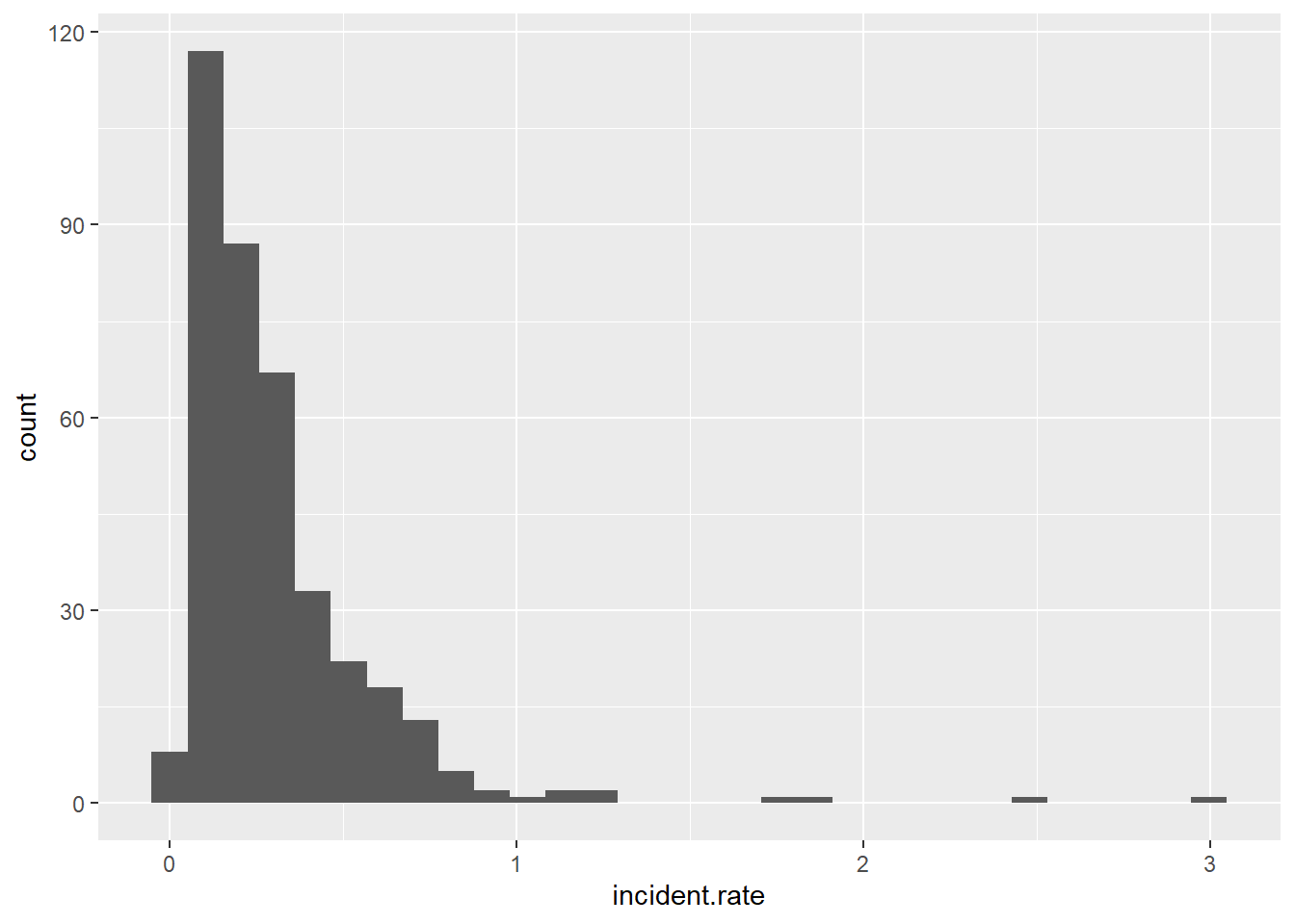
F. Homework
How many block groups have no homicides, and how many have no burglaries in 2018? What share of all block groups are these two numbers?
Make a bar chart that shows the population density (people / area) by ward. You may wish to use
st_area()to find the area of each ward. Population is already in the ward dataframe.Get two other maps (in shapefile format) not used in this tutorial. Make one ggplot with both of them, and fix the options so that it looks decent.