Loading required package: sf
Linking to GEOS 3.9.1, GDAL 3.3.2, PROJ 7.2.1; sf_use_s2() is TRUE
library(knitr)# load block group map for dc onlybg2010 <-st_read("H:/pppa_data_viz/2019/tutorial_data/lecture05/Census_Block_Groups__2010/Census_Block_Groups__2010.shp")
Reading layer `Census_Block_Groups__2010' from data source
  `H:\pppa_data_viz\2019\tutorial_data\lecture05\Census_Block_Groups__2010\Census_Block_Groups__2010.shp'
  using driver `ESRI Shapefile'
Simple feature collection with 450 features and 54 fields
Geometry type: POLYGON
Dimension:     XY
Bounding box:  xmin: -77.11976 ymin: 38.79165 xmax: -76.9094 ymax: 38.99581
Geodetic CRS:  WGS 84
# find which crimes are in which block groups# vc2010 actually already has the block group, but i want to be sure you can do this yourselfbg2010.small <- bg2010[,c("TRACT","BLKGRP","P0010001")]cbg <-st_intersection(vc2018,bg2010.small)
Warning: attribute variables are assumed to be spatially constant throughout all
geometries
head(cbg)
Simple feature collection with 6 features and 26 fields
Geometry type: POINT
Dimension:     XY
Bounding box:  xmin: -77.0734 ymin: 38.90259 xmax: -77.05759 ymax: 38.91258
Geodetic CRS:  WGS 84
           CCN               REPORT_DAT    SHIFT METHOD  OFFENSE
1826  18064713 2018-04-23T13:04:28.000Z      DAY OTHERS BURGLARY
11452 18134729 2018-08-14T03:10:42.000Z MIDNIGHT OTHERS BURGLARY
26674 18042061 2018-03-15T16:09:21.000Z  EVENING OTHERS BURGLARY
30745 18026424 2018-02-16T14:31:32.000Z      DAY OTHERS BURGLARY
30750 18026435 2018-02-16T15:42:03.000Z  EVENING OTHERS BURGLARY
23472 18136654 2018-08-17T04:38:28.000Z MIDNIGHT OTHERS BURGLARY
                                            BLOCK XBLOCK YBLOCK WARD ANC
1826             3100 - 3199 BLOCK OF K STREET NW 394626 137194    2  2E
11452            3036 - 3099 BLOCK OF M STREET NW 394737 137483    2  2E
26674            3000 - 3099 BLOCK OF N STREET NW 394778 137665    2  2E
30745 2800 - 2899 BLOCK OF PENNSYLVANIA AVENUE NW 395005 137471    2  2E
30750 2800 - 2899 BLOCK OF PENNSYLVANIA AVENUE NW 395005 137471    2  2E
23472      3700 - 3799 BLOCK OF RESERVOIR ROAD NW 393634 138304    2  2E
      DISTRICT PSA NEIGHBORHO BLOCK_GROU CENSUS_TRA VOTING_PRE LATITUDE
1826         2 206  Cluster 4   000100 4     000100 Precinct 5 38.90258
11452        2 206  Cluster 4   000100 4     000100 Precinct 5 38.90519
26674        2 206  Cluster 4   000100 4     000100 Precinct 5 38.90683
30745        2 206  Cluster 4   000100 4     000100 Precinct 5 38.90508
30750        2 206  Cluster 4   000100 4     000100 Precinct 5 38.90508
23472        2 206  Cluster 4   000201 1     000201 Precinct 6 38.91258
      LONGITUDE        BID               START_DATE                 END_DATE
1826  -77.06195 GEORGETOWN 2018-04-23T10:56:35.000Z                     <NA>
11452 -77.06068 GEORGETOWN 2018-08-13T22:52:11.000Z 2018-08-14T00:19:42.000Z
26674 -77.06021       <NA> 2018-03-14T03:48:45.000Z 2018-03-14T03:49:12.000Z
30745 -77.05759 GEORGETOWN 2018-02-16T01:25:28.000Z 2018-02-16T02:30:15.000Z
30750 -77.05759 GEORGETOWN 2018-02-15T17:30:53.000Z 2018-02-16T08:15:53.000Z
23472 -77.07340       <NA> 2018-08-17T03:36:29.000Z 2018-08-17T03:46:04.000Z
       OBJECTID  OCTO_RECOR  TRACT BLKGRP P0010001                   geometry
1826  259183436 18064713-01 000100      4     1000 POINT (-77.06196 38.90259)
11452 259193062 18134729-01 000100      4     1000  POINT (-77.06068 38.9052)
26674 259240847 18042061-01 000100      4     1000 POINT (-77.06021 38.90684)
30745 259245997 18026424-01 000100      4     1000 POINT (-77.05759 38.90509)
30750 259246002 18026435-01 000100      4     1000 POINT (-77.05759 38.90509)
23472 259224604 18136654-01 000201      1     3916  POINT (-77.0734 38.91258)
# check the sizedim(cbg)
[1] 1567 27
# get rid of geometry from points filest_geometry(cbg) <-NULL# add up to the block group levelcbg2 <-group_by(cbg, TRACT, BLKGRP, OFFENSE)cbg3 <-summarize(.data = cbg2, tot_crimes =n())
`summarise()` has grouped output by 'TRACT', 'BLKGRP'. You can override using
the `.groups` argument.
dim(cbg3)
[1] 478 4
# make crime data widecbg4 <-pivot_wider(data = cbg3,id_cols =c("TRACT","BLKGRP"),names_from = OFFENSE,values_from = tot_crimes)# check stuff head(cbg4)
# A tibble: 6 × 4
# Groups:   TRACT, BLKGRP [6]
  TRACT  BLKGRP BURGLARY HOMICIDE
  <chr>  <chr>     <int>    <int>
1 000100 2             1       NA
2 000100 3             1       NA
3 000100 4             5       NA
4 000201 1             3       NA
5 000202 1             2       NA
6 000202 2             2       NA
dim(cbg4)
[1] 387 4
# merge each back into the block groups file so we have all block groups with shapes and populationbg2010.c2 <-merge(x = bg2010.small, y = cbg4, by =c("TRACT","BLKGRP"), all =TRUE)dim(bg2010.c2)
[1] 450 6
# --- make quartiles for homicides# make NA values zerobg2010.c2$HOMICIDE <-ifelse(test =is.na(bg2010.c2$HOMICIDE) ==TRUE,yes =0,no = bg2010.c2$HOMICIDE)# make quartilesbg2010.c2$hom.quartile2 <-ntile(bg2010.c2$HOMICIDE, 4)# checktable(bg2010.c2$hom.quartile2)
  1   2   3   4
113 113 112 112
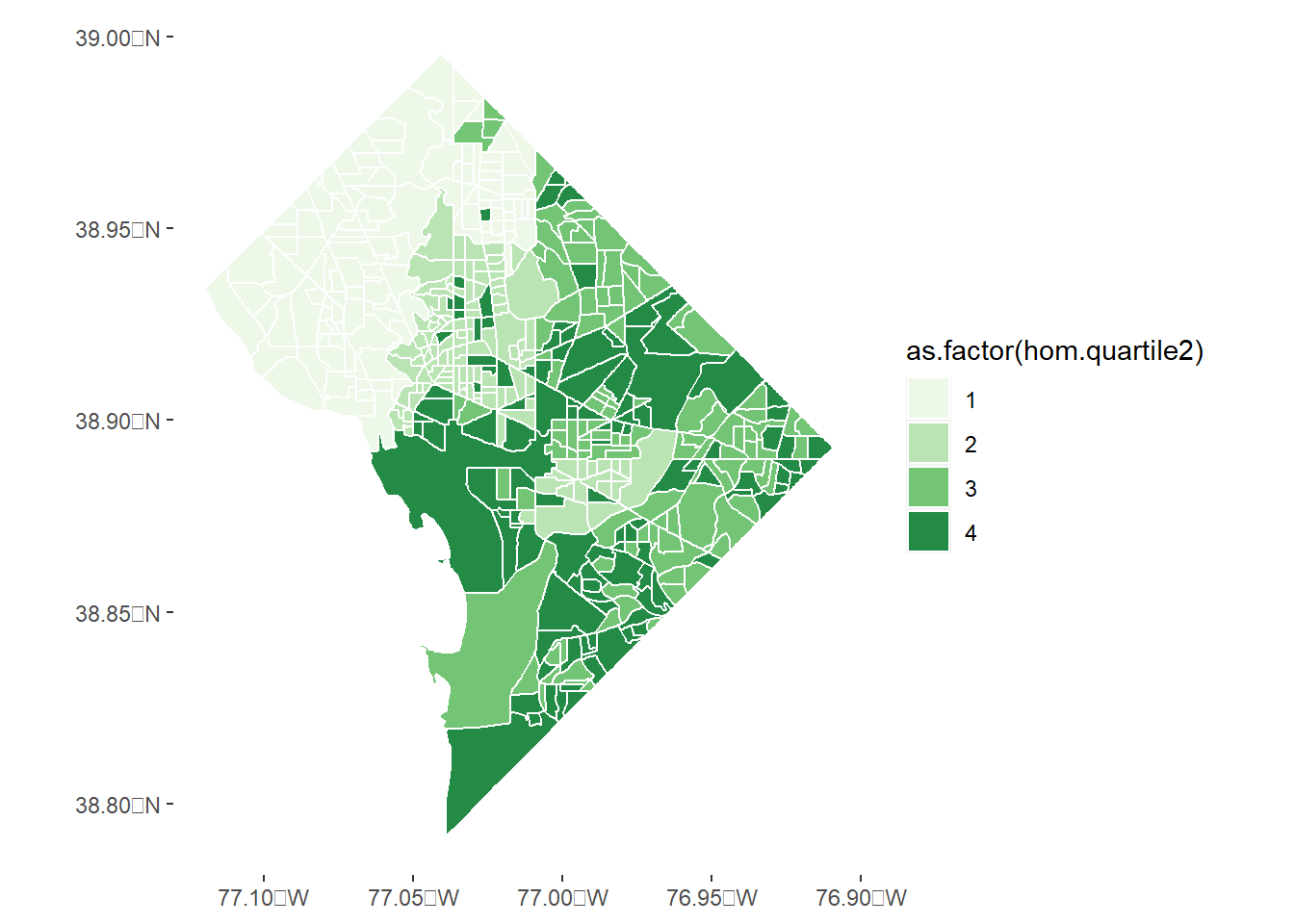
# make color ramp# see four.colors <-c("#edf8e9","#bae4b3","#74c476","#238b45")# homicide choroplethhomc <-ggplot() +geom_sf(data = bg2010.c2, mapping =aes(fill =as.factor(hom.quartile2)), color ="white") +scale_fill_manual(values = four.colors) +theme(panel.background =element_rect(fill ="transparent",colour =NA),plot.background =element_rect(fill ="transparent",colour =NA))homc
There are many ways to improve this chart, but one thing that bothered me quite a bit was that the distribution of homicides overlapped by quartile. Fundamentally, using quartiles here was a poor choice.
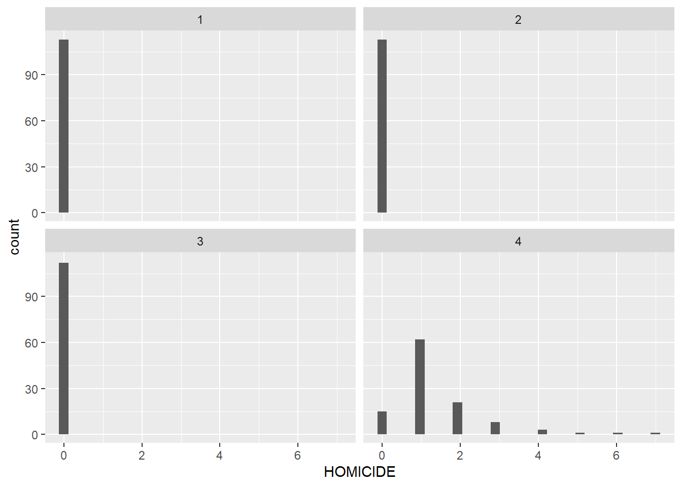
Here’s how I show that quartiles are a poor choice:
# make a facet wrapped histogram to show troubles with distributionbarso <-ggplot() +geom_histogram(data = bg2010.c2,mapping =aes(x = HOMICIDE)) +facet_wrap(~hom.quartile2)barso
`stat_bin()` using `bins = 30`. Pick better value with `binwidth`.
The first, second and third quartiles are all zeros!
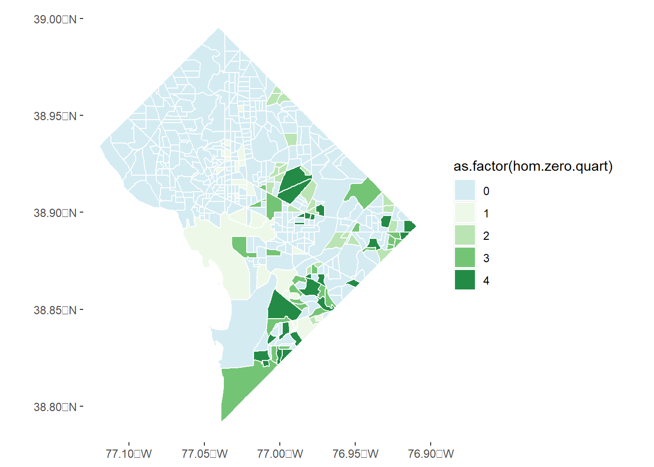
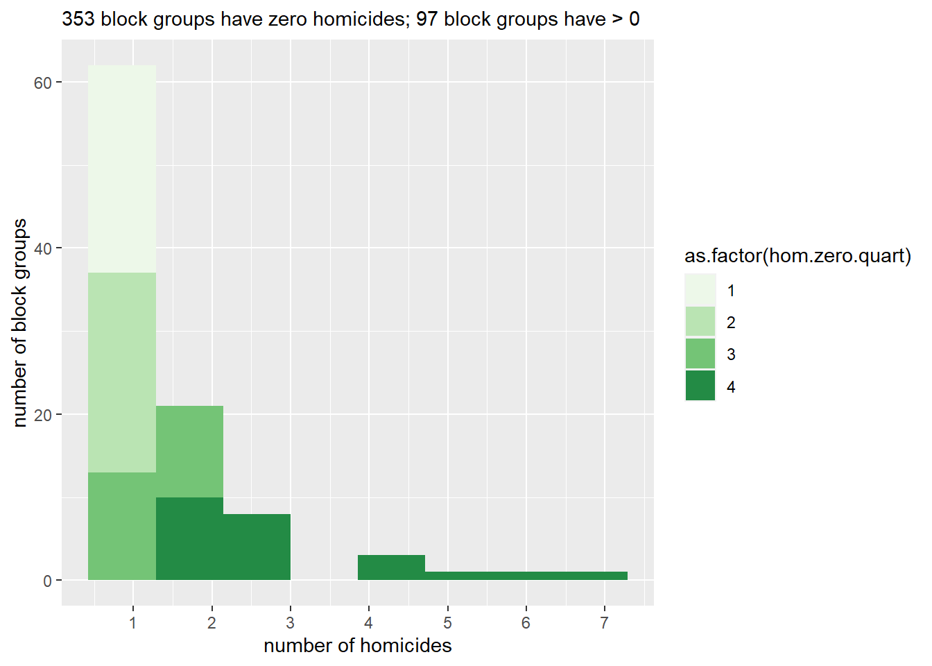
Here’s a slight improvement. I separate out the zero block groups from the non-zero block groups, and then plot the map again. I then follow with a histogram legend.. which shows that maybe I still need to make some fixes, since the first, second, and part of the third quartiles are all block groups with 1 homicide. However, this second one is clearly better than the first.
# ---- now lets make a better version# first a marker for whether homicides are zerobg2010.c2$not.zero.hom <-ifelse(test = bg2010.c2$HOMICIDE ==0,yes =0, no =1)# now make a quartile for each of these two groups -- zeros and non-zeros# just keep in mind that the quartiles for the zeros are garbage, b/c all obs are zero!bg2010.c2 <-group_by(.data = bg2010.c2, not.zero.hom)bg2010.c2 <-mutate(.data = bg2010.c2,not.zero.hom.q =ntile(HOMICIDE, n =4))table(bg2010.c2$not.zero.hom.q)
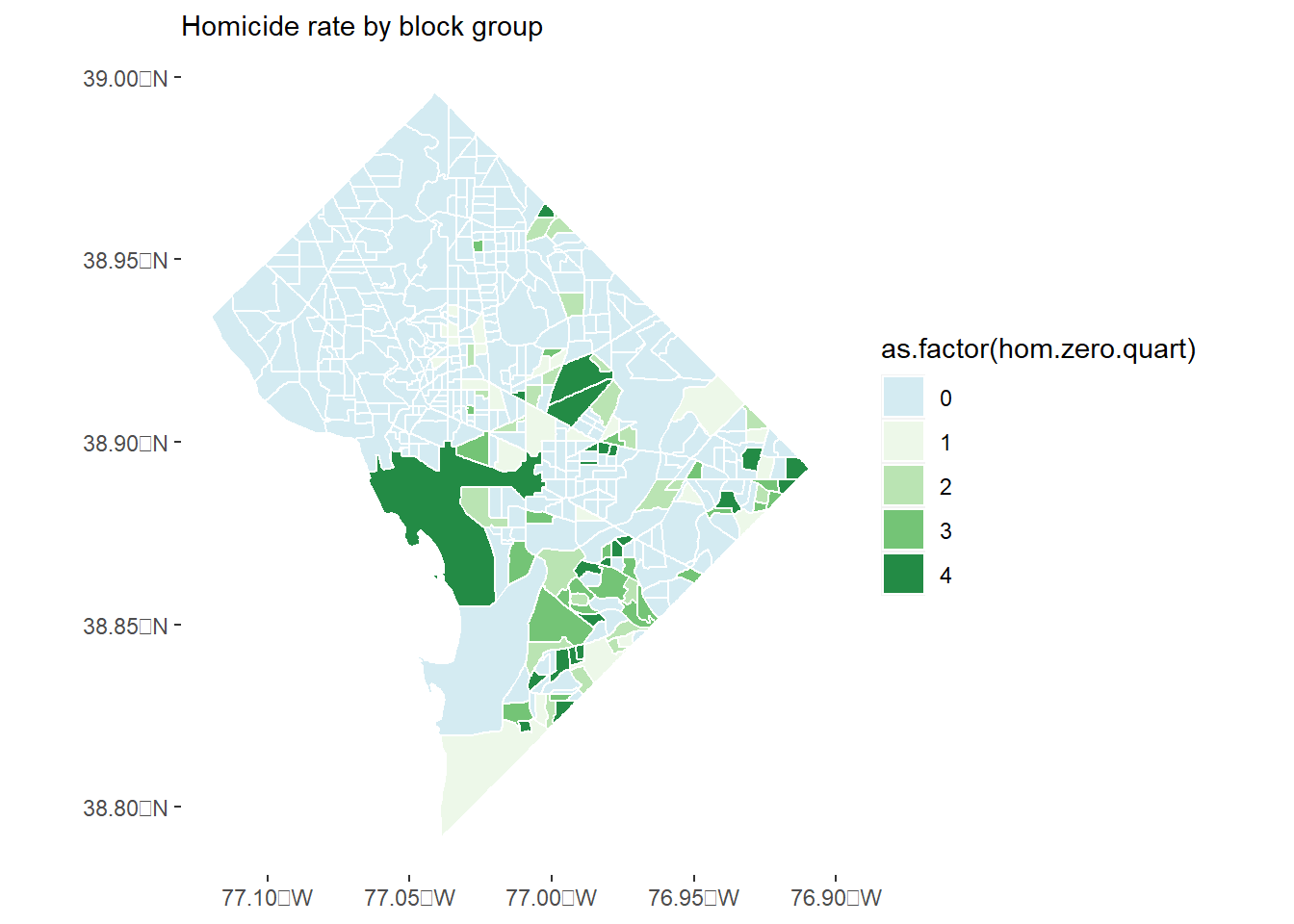
# now make a final variable that is zero if there are zero homicides and the quartile number if# there are non-zero homicides# this is the not.zero.hom (0/1) * quartile by groupbg2010.c2$hom.zero.quart <- bg2010.c2$not.zero.hom*bg2010.c2$not.zero.hom.q# now re-do the map with this new variable and a new light blue color for the zerosc0 <-"#d4ebf2"homc <-ggplot() +geom_sf(data = bg2010.c2, mapping =aes(fill =as.factor(hom.zero.quart)), color ="white") +scale_fill_manual(values =c(c0,four.colors)) +theme(panel.background =element_rect(fill ="transparent",colour =NA),plot.background =element_rect(fill ="transparent",colour =NA))homc
# and a little histogram legend# find no. of block groups with and without homicides# no homicidesbg.no.hom <-nrow(filter(.data = bg2010.c2, HOMICIDE ==0))bg.hom <-nrow(filter(.data = bg2010.c2, HOMICIDE >0))barso <-ggplot() +geom_histogram(data =filter(.data = bg2010.c2, HOMICIDE >0),mapping =aes(x = HOMICIDE, fill =as.factor(hom.zero.quart)),bins =8) +scale_fill_manual(values =c(four.colors)) +scale_x_continuous(breaks =c(seq(1,8,1)), labels =c(seq(1,8,1))) +#scale_y_continuous(labels = c(seq(1,8,1), breaks = c(seq(1,8,1))) +labs(subtitle =paste0(bg.no.hom," block groups have zero homicides; ", bg.hom, " block groups have > 0"),y ="number of block groups",x ="number of homicides")barso
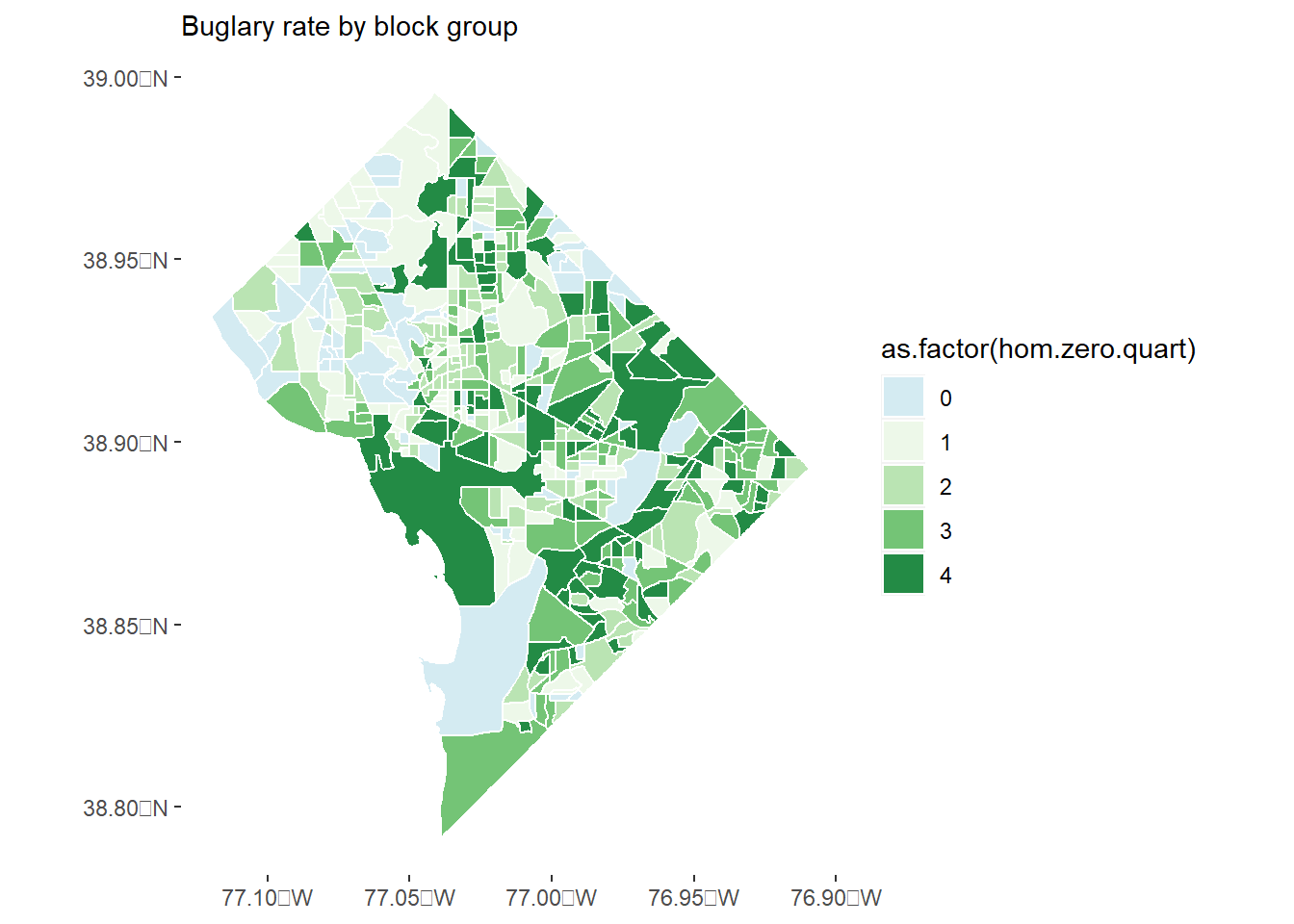
Make choropleths for both homicides and burglaries in rates (per residential population). Recall that population is in bg2010 when you load it.
Answer:
# make NA values zerobg2010.c2$BURGLARY <-ifelse(test =is.na(bg2010.c2$BURGLARY) ==TRUE,yes =0,no = bg2010.c2$BURGLARY)# make choropleths for burglaries and homicides in rateschoro.maker <-function(varin, varname){# calculate rate of variableprint("beginning of function")print(names(bg2010.c2)) bg2010.c2$rate <- bg2010.c2[[varin]] / bg2010.c2$P0010001print(summary(bg2010.c2$rate))# first a marker for whether the rate is zeroprint("before marker") bg2010.c2$not.zero.hom <-ifelse(test = bg2010.c2$rate ==0,yes =0, no =1)# now make a quartile for each of these two groups -- zeros and non-zeros# just keep in mind that the quartiles for the zeros are garbage, b/c all obs are zero!print("before group_by") bg2010.c2 <-group_by(.data = bg2010.c2, not.zero.hom) bg2010.c2 <-mutate(.data = bg2010.c2,not.zero.hom.q =ntile(rate, n =4))# now make a final variable that is zero if there are zero homicides and the quartile number if# there are non-zero homicides# this is the not.zero.hom (0/1) * quartile by group bg2010.c2$hom.zero.quart <- bg2010.c2$not.zero.hom*bg2010.c2$not.zero.hom.q# now make a choropleth of these guys homc <-ggplot() +geom_sf(data = bg2010.c2, mapping =aes(fill =as.factor(hom.zero.quart)), color ="white") +scale_fill_manual(values =c(c0,four.colors)) +theme(panel.background =element_rect(fill ="transparent",colour =NA),plot.background =element_rect(fill ="transparent",colour =NA)) +labs(subtitle =paste0(varname, " rate by block group"))print(homc)return(homc) } # end of function to make choropleth for rates# run this functiong0 <-choro.maker(varin ="HOMICIDE", varname ="Homicide")
[1] "beginning of function"
 [1] "TRACT"          "BLKGRP"         "P0010001"       "BURGLARY"
 [5] "HOMICIDE"       "geometry"       "hom.quartile2"  "not.zero.hom"
 [9] "not.zero.hom.q" "hom.zero.quart"
     Min.   1st Qu.    Median      Mean   3rd Qu.      Max.
0.0000000 0.0000000 0.0000000 0.0003333 0.0000000 0.0303030
[1] "before marker"
[1] "before group_by"
[1] "beginning of function"
 [1] "TRACT"          "BLKGRP"         "P0010001"       "BURGLARY"
 [5] "HOMICIDE"       "geometry"       "hom.quartile2"  "not.zero.hom"
 [9] "not.zero.hom.q" "hom.zero.quart"
     Min.   1st Qu.    Median      Mean   3rd Qu.      Max.
0.0000000 0.0008722 0.0018753 0.0025883 0.0033515 0.0303030
[1] "before marker"
[1] "before group_by"
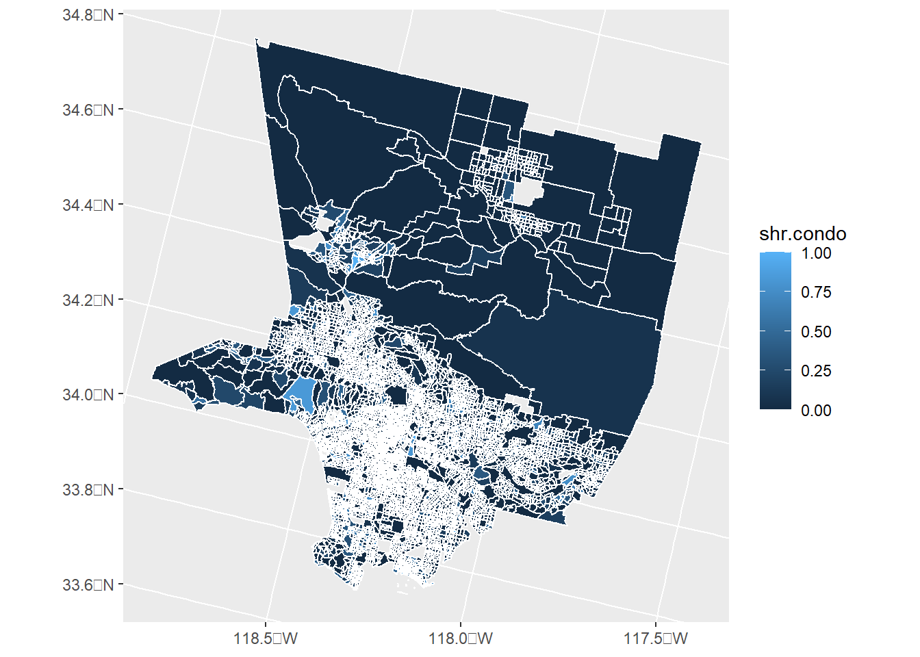
Pull in other geographic data (the data we used earlier this semester is fine, as is any other of your choice) and make a choropleth map with a histogram legend.
Answer:
Here I am using some data I created for a project I’m working on about condominiums. I first look at the distribution and then decide how to create the categories.
# read the block group data I created elsewherefn <-"H:/condos/r_output/la_condo_exploration/condos_by_blockgroup_20230331.rds"bg.data <-readRDS(fn)# read the block group mapfn <-"H:/maps/united_states/census2020/block_groups/nhgis0001_shape/US_blck_grp_2020.shp"us.bg.map <-st_read(fn)
Reading layer `US_blck_grp_2020' from data source
  `H:\maps\united_states\census2020\block_groups\nhgis0001_shape\US_blck_grp_2020.shp'
  using driver `ESRI Shapefile'
Simple feature collection with 241764 features and 15 fields
Geometry type: MULTIPOLYGON
Dimension:     XY
Bounding box:  xmin: -7115208 ymin: -1685018 xmax: 3321632 ymax: 4591848
Projected CRS: USA_Contiguous_Albers_Equal_Area_Conic
# cut to just la county bg.map.la <- us.bg.map[which(us.bg.map$STATE =="06"& us.bg.map$COUNTY =="037"),]# merge the two of thembg.both <-merge(x = bg.map.la,y = bg.data,by =c("TRACTCE","BLKGRPCE"),all =TRUE)# check on the mergedim(bg.map.la)
[1] 6587 16
dim(bg.data)
[1] 6588 10
dim(bg.both)
[1] 6588 24
# lets get rid of all ratios that are > 1bg.both[which(bg.both$shr.condo >1),]
# make a choroplethchoro <-ggplot() +geom_sf(data = bg.both,mapping =aes(fill = shr.condo),color ="white")choro
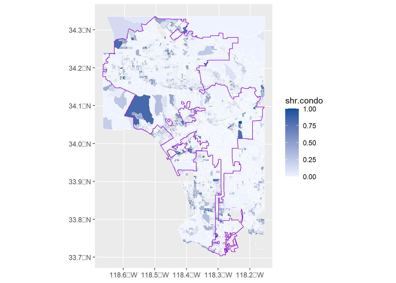
But this graph is really awful! Mostly white lines. So here is a fixed version. I focus just on the city of Los Angeles and I make some modifications to the color scheme.
# read in shape file with all incorporated municipalities in LA countycity.map.file <-"H:/maps/los_angeles/city_boundaries/20101220_inc_cities_only.shp"city.map <-st_read(city.map.file)
Reading layer `20101220_inc_cities_only' from data source
  `H:\maps\los_angeles\city_boundaries\20101220_inc_cities_only.shp'
  using driver `ESRI Shapefile'
Simple feature collection with 104 features and 20 fields
Geometry type: POLYGON
Dimension:     XY
Bounding box:  xmin: 6281837 ymin: 1574188 xmax: 6659162 ymax: 2102434
Projected CRS: NAD83 / California zone 5 (ftUS)
head(city.map)
Simple feature collection with 6 features and 20 fields
Geometry type: POLYGON
Dimension:     XY
Bounding box:  xmin: 6390856 ymin: 1922165 xmax: 6586892 ymax: 2102434
Projected CRS: NAD83 / California zone 5 (ftUS)
  OBJECTID AREA    PERIMETER GPLAN_INDE GPLAN_IN_1 CITY    CITYNAME_A
1        1    0 678822.57063          2          2 1418     LANCASTER
2        8    0 679381.41469          9         10 1971      PALMDALE
3       17    0   9495.81762         18         22 2356 SANTA CLARITA
4       18    0     16.42616         19         22 2356 SANTA CLARITA
5       19    0   2673.60151         20         22 2356 SANTA CLARITA
6       23    0  36599.03312         24         25 2316  SAN FERNANDO
  SYMBOL_COL COMP_NO TYPE ADOPTED SYMBOL NAME   ACRES    CITY_COMM_ ZCIP_PHASE
1         13       0 <NA>    <NA>     13 <NA> 60489.5     LANCASTER       <NA>
2         67       0 <NA>    <NA>     67 <NA> 67951.7      PALMDALE       <NA>
3         25       0 <NA>    <NA>     25 <NA>    54.0 SANTA CLARITA       <NA>
4         25       0 <NA>    <NA>     25 <NA>     0.0 SANTA CLARITA       <NA>
5         25       0 <NA>    <NA>     25 <NA>     6.1 SANTA CLARITA       <NA>
6         25       0 <NA>    <NA>     25 <NA>  1518.2  SAN FERNANDO       <NA>
  SQ_MILES        JURISDICTI   Shape_area    Shape_len
1   94.515 INCORPORATED CITY 2.634923e+09 678822.57355
2  106.174 INCORPORATED CITY 2.959975e+09 679381.41837
3    0.084 INCORPORATED CITY 2.352046e+06   9495.81836
4    0.000 INCORPORATED CITY 1.187475e+01     16.42601
5    0.009 INCORPORATED CITY 2.636935e+05   2673.60099
6    2.372 INCORPORATED CITY 6.613310e+07  36599.03420
                        geometry
1 POLYGON ((6500775 2066684, ...
2 POLYGON ((6577419 2062852, ...
3 POLYGON ((6393158 1953813, ...
4 POLYGON ((6394042 1953301, ...
5 POLYGON ((6393931 1952652, ...
6 POLYGON ((6430051 1932497, ...
# make just la city mapla <- city.map[which(city.map$CITYNAME_A =="LOS ANGELES"),]# chop the block group maps to the bounding box of the city of los angeles# but first give block group map same projection as la city mapbg.both <-st_transform(bg.both, crs =st_crs(la))la.bgs.only <-st_crop(x = bg.both, y =st_bbox(la))
Warning: attribute variables are assumed to be spatially constant throughout all
geometries
# now re-do choropleth with just city of lachoro <-ggplot() +geom_sf(data = la.bgs.only,mapping =aes(fill = shr.condo),color ="white",size =0.2) +geom_sf(data = la,fill ="transparent",color ="purple") +scale_fill_continuous(high ="#08519c", low ="#eff3ff")choro
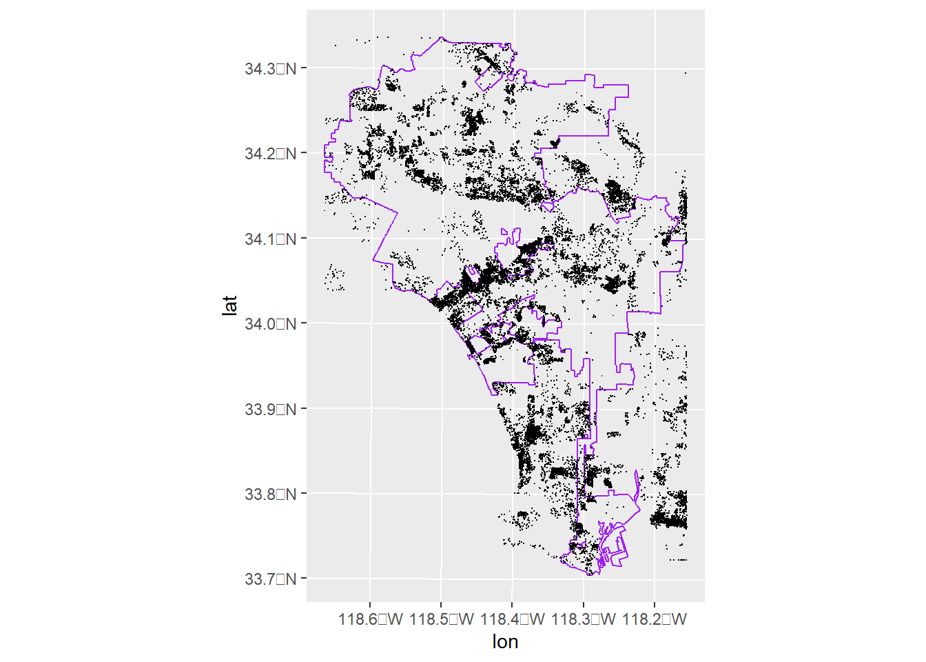
Make a dot density map with the data of your choice and at least two groups.
Answer:
Here I am showing a dot density map with one group – condos in LA. I don’t have an obvious second group in these data, but this should be enough to figure out how to do two groups if you wanted to.
# we'll use the la cit block group map from above# lets plot condos in red and plot one dot for each condola.bgs.only$ten.condos <- la.bgs.only$num.condos /10# if less than 0.1, assign zerola.bgs.only$ten.condos <-ifelse(test = (la.bgs.only$ten.condos <1& la.bgs.only$ten.condos >0),yes =1,no = la.bgs.only$ten.condos)la.bgs.only$ten.condos.int <-as.integer(la.bgs.only$ten.condos)print("this is the thing to make dots from")
# get the points to plothdots <-st_sample(x = la.bgs.only, size = la.bgs.only$ten.condos.int, type ="random", progress =TRUE)hdots <-st_cast(x = hdots, to ="POINT")hdots.mat <-st_coordinates(hdots)hdats.df <-as.data.frame(hdots.mat)hdats.df <-setNames(object = hdats.df, nm =c("lon","lat"))# plot these dots with an la map county map behind it# make the plotdotso <-ggplot() +geom_sf(data = la,fill ="transparent",color ="purple") +geom_point(data = hdats.df,mapping =aes(x=lon, y = lat),shape =".")dotso