summer(x = 1, y = 2)
summer(x = 2, y = 1)Tutorial 6 Answers
Problem Set 6: Questions and Answers
- In section B.1., why do
not yield the same output? Write in math what each one does.
Answer:
Both functions calculate \[x^y\]. Therefore, the first function evaluates to \(1^2\), which is equal to 1. The second function evaluates to \(2^1\), which is equal to 2.
- In section C.1., why does the call
summer3(x = 5, y = 3)return a value whensummer2(x = 5, y = 3)does not?
Answer:
The function summer2 requires a value for z so summer2(x = 5, y = 3) breaks.
The function summer3 can accept a z values, but R does not need a value for z1 to evaluate the function. Therefore,summer3(x = 5, y = 3)` works without error.
- In C.2., why does
summer(x = "fred", y = "ted")yield an error?
Answer:
The function summer uses x and y as numeric variables in a function. Therefore, when you try to do \[\text{fred}^{\text{ted}}\] R gets confused and breaks.
- Fix the function in part F to remove the graph background. In
ggplotwe remove the grey background by adding to the theme element:
plotto <- ggplot() +
  geom_whatever(data = df,
                mapping = aes(x = var, y = yvar)) +
  theme(panel.background = element_blank())
You can also get rid of the gridlines with
  theme(panel.background = element_blank(),
        panel.grid.major = element_blank(),
        panel.grid.minor = element_blank())
Answer: The original function was
library(tidyverse)── Attaching packages ─────────────────────────────────────── tidyverse 1.3.1 ──✔ ggplot2 3.3.6 ✔ purrr 0.3.4
✔ tibble 3.1.7 ✔ dplyr 1.0.9
✔ tidyr 1.2.0 ✔ stringr 1.4.0
✔ readr 2.1.2 ✔ forcats 0.5.1── Conflicts ────────────────────────────────────────── tidyverse_conflicts() ──
✖ dplyr::filter() masks stats::filter()
✖ dplyr::lag() masks stats::lag()# load data
crashes <- read.csv("H:/pppa_data_viz/2023/tutorials/data/tutorial_06/20230307_Crashes_in_DC.csv")
# graphing function
graphit2 <- function(xvar,namer1){
ggplot() +
geom_histogram(data = crashes,
mapping = aes(x = {{xvar}})) +
labs(title = paste0("Histogram of ",namer1),
x = namer1)
}
# call the graphing function
graphit2(xvar = TOTAL_VEHICLES, namer1 = "total vehicles involved in crash")`stat_bin()` using `bins = 30`. Pick better value with `binwidth`.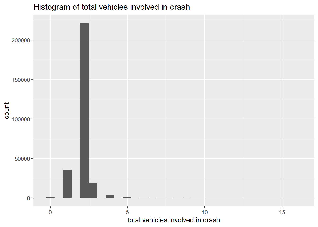
We modify by adding theme elements:
graphit2 <- function(xvar,namer1){
  ggplot() +
    geom_histogram(data = crashes,
         mapping = aes(x = {{xvar}})) +
    labs(title = paste0("Histogram of ",namer1),
         x = namer1) +
    theme(panel.background = element_blank(),
        panel.grid.major = element_blank(),
        panel.grid.minor = element_blank())
}
graphit2(xvar = TOTAL_VEHICLES, namer1 = "total vehicles involved in crash")
`stat_bin()` using `bins = 30`. Pick better value with `binwidth`.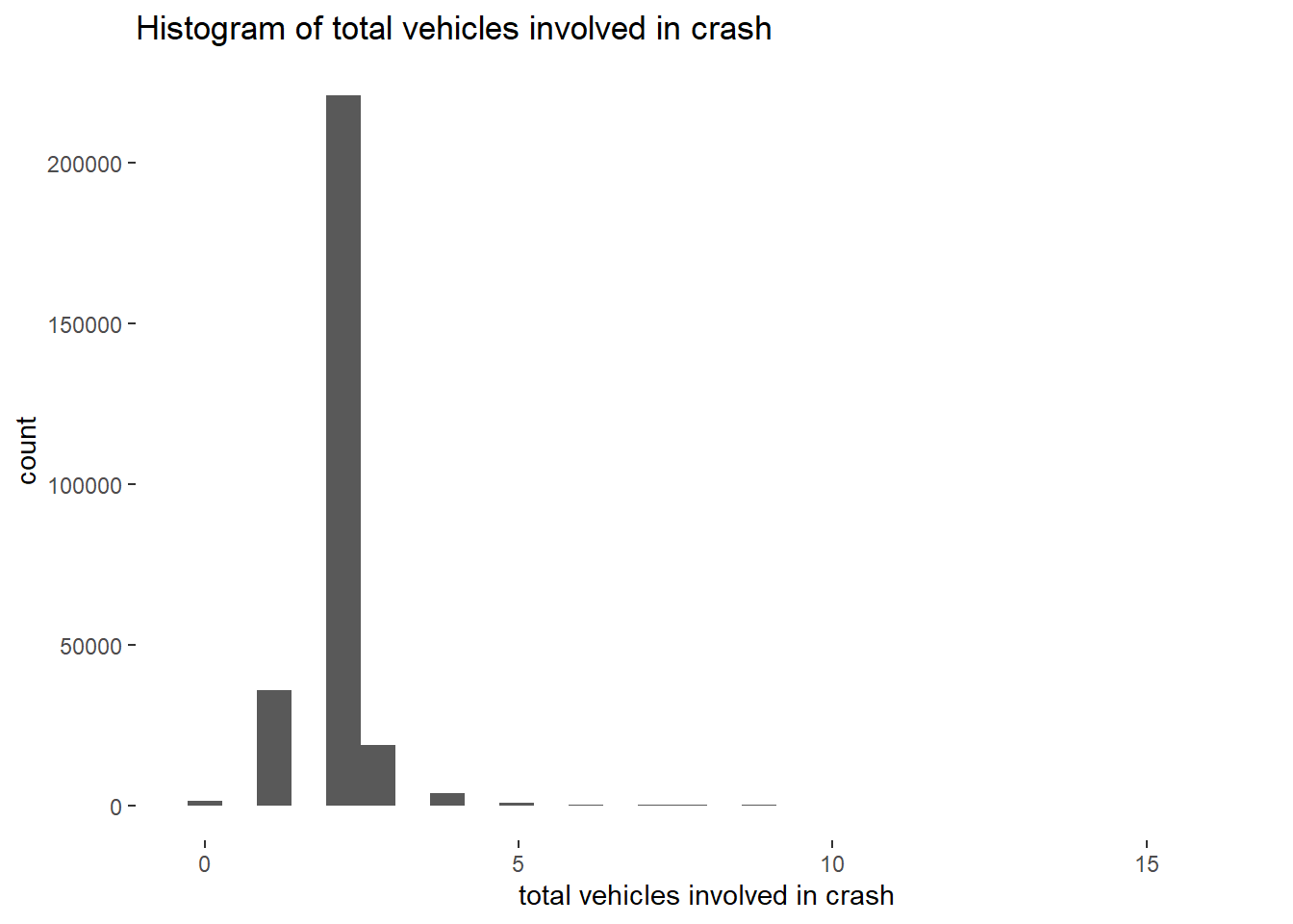
- Make a function that automates a graphics operation of interest to you, using a dataset not from this tutorial.
Answer:
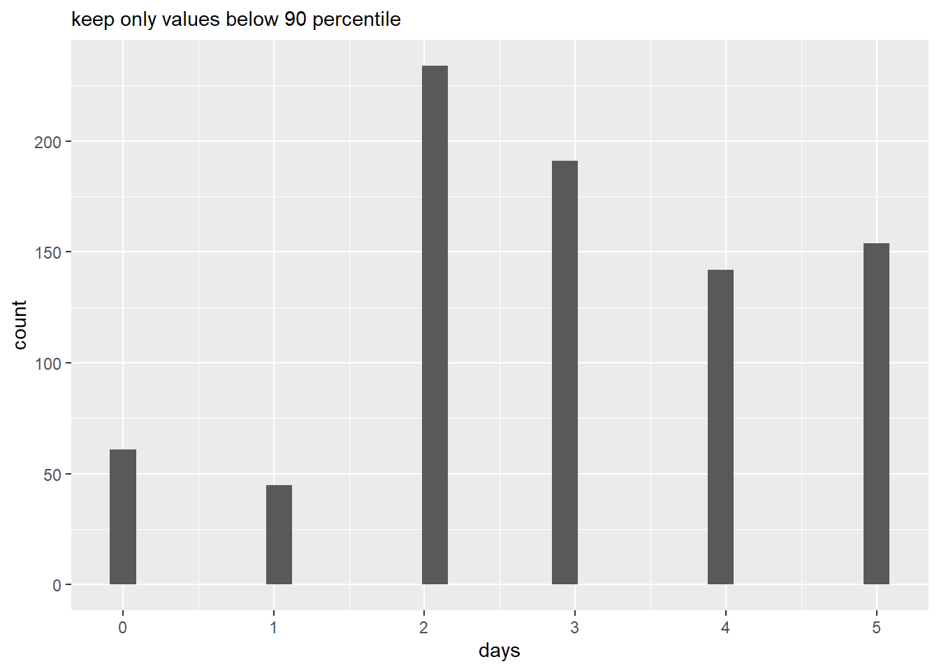
Here is one example, using 311 data from the city of Los Angeles. I think that my histogram with the full distribution of values looks bad because of a few very high values. I use a function to make a variety of graphs dropping values above the 99th, 95th and 90th percentiles, sequentially.
# location of la's 311 data for 2022
# https://data.lacity.org/City-Infrastructure-Service-Requests/MyLA311-Service-Request-Data-2022/i5ke-k6by
three11 <- "https://data.lacity.org/resource/i5ke-k6by.csv"

# load the data
la3 <- read_csv(three11)
Rows: 1000 Columns: 34
── Column specification ────────────────────────────────────────────────────────
Delimiter: ","
chr (26): SRNumber, CreatedDate, UpdatedDate, ActionTaken, Owner, RequestTyp...
dbl (8): HouseNumber, ZipCode, Latitude, Longitude, TBMPage, TBMRow, CD, NC
ℹ Use `spec()` to retrieve the full column specification for this data.
ℹ Specify the column types or set `show_col_types = FALSE` to quiet this message.str(la3)spec_tbl_df [1,000 × 34] (S3: spec_tbl_df/tbl_df/tbl/data.frame)
$ SRNumber : chr [1:1000] "1-2154996101" "1-2154995181" "1-2154996311" "1-2154996331" ...
$ CreatedDate : chr [1:1000] "01/01/2022 12:08:14 AM" "01/01/2022 12:15:59 AM" "01/01/2022 12:24:31 AM" "01/01/2022 12:24:38 AM" ...
$ UpdatedDate : chr [1:1000] "01/03/2022 10:39:18 PM" "01/01/2022 01:06:13 PM" "01/03/2022 12:21:42 AM" "01/03/2022 09:37:09 AM" ...
$ ActionTaken : chr [1:1000] "SR Created" "SR Created" "SR Created" "SR Created" ...
$ Owner : chr [1:1000] "LASAN" "LASAN" "LASAN" "LASAN" ...
$ RequestType : chr [1:1000] "Bulky Items" "Dead Animal Removal" "Bulky Items" "Metal/Household Appliances" ...
$ Status : chr [1:1000] "Closed" "Closed" "Cancelled" "Cancelled" ...
$ RequestSource : chr [1:1000] "Self Service" "Call" "Self Service" "Self Service" ...
$ CreatedByUserOrganization: chr [1:1000] "Self Service_SAN" "LASAN" "Self Service" "Self Service_SAN" ...
$ MobileOS : chr [1:1000] NA NA NA NA ...
$ Anonymous : chr [1:1000] "N" "N" "N" "N" ...
$ AssignTo : chr [1:1000] "WLA" "HB" "EV" "WV" ...
$ ServiceDate : chr [1:1000] "01/03/2022 12:00:00 AM" NA "01/05/2022 12:00:00 AM" "01/04/2022 12:00:00 AM" ...
$ ClosedDate : chr [1:1000] "01/03/2022 02:58:20 PM" "01/01/2022 01:06:13 PM" "01/03/2022 12:21:40 AM" "01/03/2022 09:37:08 AM" ...
$ AddressVerified : chr [1:1000] "Y" "Y" "Y" "Y" ...
$ ApproximateAddress : chr [1:1000] "N" "N" "N" "N" ...
$ Address : chr [1:1000] "4776 S LA VILLA MARINA, 90292" "HOOVER ST AT IMPERIAL HWY, 90044" "4144 N TUJUNGA AVE, 91604" "10118 N LURLINE AVE, 91311" ...
$ HouseNumber : num [1:1000] 4776 NA 4144 10118 17101 ...
$ Direction : chr [1:1000] "S" NA "N" "N" ...
$ StreetName : chr [1:1000] "LA VILLA MARINA" NA "TUJUNGA" "LURLINE" ...
$ Suffix : chr [1:1000] NA NA "AVE" "AVE" ...
$ ZipCode : num [1:1000] 90292 90044 91604 91311 91344 ...
$ Latitude : num [1:1000] 34 33.9 34.1 34.3 34.3 ...
$ Longitude : num [1:1000] -118 -118 -118 -119 -119 ...
$ Location : chr [1:1000] "(33.9812287953, -118.433950454)" "(33.930968583, -118.286997573)" "(34.1436314704, -118.378844267)" "(34.2540709722, -118.584098582)" ...
$ TBMPage : num [1:1000] 672 704 562 500 481 594 501 501 501 501 ...
$ TBMColumn : chr [1:1000] "C" "B" "J" "C" ...
$ TBMRow : num [1:1000] 7 6 5 4 6 6 2 2 2 2 ...
$ APC : chr [1:1000] "West Los Angeles APC" "South Los Angeles APC" "South Valley APC" "North Valley APC" ...
$ CD : num [1:1000] 11 8 2 12 12 13 12 12 12 12 ...
$ CDMember : chr [1:1000] "Mike Bonin" "Marqueece Harris-Dawson" "Paul Krekorian" "John Lee" ...
$ NC : num [1:1000] 70 90 27 99 4 38 118 118 118 118 ...
$ NCName : chr [1:1000] "Del Rey" "Harbor Gateway North" "Studio City" "Chatsworth" ...
$ PolicePrecinct : chr [1:1000] "PACIFIC" "SOUTHEAST" "NORTH HOLLYWOOD" "DEVONSHIRE" ...
- attr(*, "spec")=
.. cols(
.. SRNumber = col_character(),
.. CreatedDate = col_character(),
.. UpdatedDate = col_character(),
.. ActionTaken = col_character(),
.. Owner = col_character(),
.. RequestType = col_character(),
.. Status = col_character(),
.. RequestSource = col_character(),
.. CreatedByUserOrganization = col_character(),
.. MobileOS = col_character(),
.. Anonymous = col_character(),
.. AssignTo = col_character(),
.. ServiceDate = col_character(),
.. ClosedDate = col_character(),
.. AddressVerified = col_character(),
.. ApproximateAddress = col_character(),
.. Address = col_character(),
.. HouseNumber = col_double(),
.. Direction = col_character(),
.. StreetName = col_character(),
.. Suffix = col_character(),
.. ZipCode = col_double(),
.. Latitude = col_double(),
.. Longitude = col_double(),
.. Location = col_character(),
.. TBMPage = col_double(),
.. TBMColumn = col_character(),
.. TBMRow = col_double(),
.. APC = col_character(),
.. CD = col_double(),
.. CDMember = col_character(),
.. NC = col_double(),
.. NCName = col_character(),
.. PolicePrecinct = col_character()
.. )
- attr(*, "problems")=<externalptr> # --- calculate the length of time from start to close
# start date
la3$start.date <- as.Date(x = substr(la3$CreatedDate, start = 1, stop = 10), format = "%m/%d/%Y")
# stop date
la3$stop.date <- as.Date(x = substr(la3$ClosedDate, start = 1, stop = 10), format = "%m/%d/%Y")
# number of days between these two
la3$days <- la3$stop.date - la3$start.date
# double-check it
table(la3$days)
  0   1   2   3   4   5   6   7   8   9  10  11  12  13  17  18  19  24  25  32
 61  45 234 191 142 154  74  29   4  10   5   4   3   2   2   1   1   4   6   1
 36  37  40  43  44  45  54  59  78  96  97 101 120 163 174 325 423
  5   1   1   1   1   1   1   1   1   1   2   2   1   1   1   1   2
# -- function to see how the distribution looks when I cut off parts at the top
histo <- function(topcoder){
# find the value of the percentile in the function
qer <- quantile(x = la3$days, probs = c(topcoder), na.rm = TRUE)
# keep only data below this value
la3.limit <- filter(la3, days < qer)
# make a histogram
la.hist <- ggplot() +
geom_histogram(data = la3.limit,
mapping = aes(x = days)) +
labs(subtitle = paste0("keep only values below ",topcoder*100," percentile"))
print(la.hist)
}
# --- call the function for various top-coding values
# drop above 99th p
histo(topcoder = 0.99)Don't know how to automatically pick scale for object of type difftime. Defaulting to continuous.
`stat_bin()` using `bins = 30`. Pick better value with `binwidth`.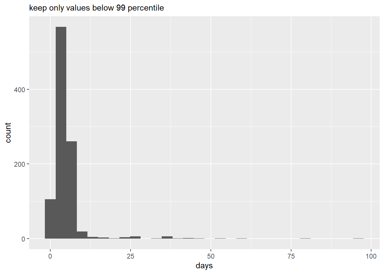
# drop above 95th p
histo(topcoder = 0.95)
Don't know how to automatically pick scale for object of type difftime. Defaulting to continuous.
`stat_bin()` using `bins = 30`. Pick better value with `binwidth`.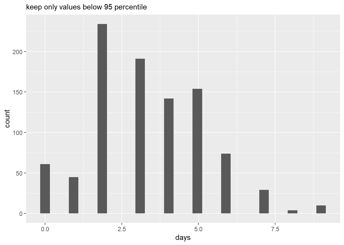
# drop above 90th p
histo(topcoder = 0.90)
Don't know how to automatically pick scale for object of type difftime. Defaulting to continuous.
`stat_bin()` using `bins = 30`. Pick better value with `binwidth`.