Tutorial 5 Answers

Problem Set 5: Questions and Answers

  1. How many block groups have no homicides, and how many have no burglaries in 2018? What share of all block groups are these two numbers?

Answer:

# libraries
library(tidyverse)
── Attaching packages ─────────────────────────────────────── tidyverse 1.3.2 ──
✔ ggplot2 3.3.6     ✔ purrr   0.3.4
✔ tibble  3.1.7     ✔ dplyr   1.0.9
✔ tidyr   1.2.0     ✔ stringr 1.4.0
✔ readr   2.1.2     ✔ forcats 0.5.1
── Conflicts ────────────────────────────────────────── tidyverse_conflicts() ──
✖ dplyr::filter() masks stats::filter()
✖ dplyr::lag()    masks stats::lag()
library(sf)
Linking to GEOS 3.9.1, GDAL 3.3.2, PROJ 7.2.1; sf_use_s2() is TRUE
# --- first, figure out the # of homicides and burglaries by block group

# load crime data
c2018 <- st_read("H:/pppa_data_viz/2019/tutorial_data/lecture05/Crime_Incidents_in_2018/Crime_Incidents_in_2018.shp")
Reading layer `Crime_Incidents_in_2018' from data source 
  `H:\pppa_data_viz\2019\tutorial_data\lecture05\Crime_Incidents_in_2018\Crime_Incidents_in_2018.shp' 
  using driver `ESRI Shapefile'
Simple feature collection with 33645 features and 23 fields
Geometry type: POINT
Dimension:     XY
Bounding box:  xmin: -77.11232 ymin: 38.81467 xmax: -76.91002 ymax: 38.9937
Geodetic CRS:  WGS 84
# make smaller dataframe -- just homicides and burglaries
vc2018 <- c2018[which(c2018$OFFENSE == "HOMICIDE" | c2018$OFFENSE == "BURGLARY"),]

# load block group map
bg2010 <- st_read("H:/pppa_data_viz/2019/tutorial_data/lecture05/Census_Block_Groups__2010/Census_Block_Groups__2010.shp")
Reading layer `Census_Block_Groups__2010' from data source 
  `H:\pppa_data_viz\2019\tutorial_data\lecture05\Census_Block_Groups__2010\Census_Block_Groups__2010.shp' 
  using driver `ESRI Shapefile'
Simple feature collection with 450 features and 54 fields
Geometry type: POLYGON
Dimension:     XY
Bounding box:  xmin: -77.11976 ymin: 38.79165 xmax: -76.9094 ymax: 38.99581
Geodetic CRS:  WGS 84
names(bg2010)
 [1] "OBJECTID"   "TRACT"      "BLKGRP"     "GEOID"      "P0010001"  
 [6] "P0010002"   "P0010003"   "P0010004"   "P0010005"   "P0010006"  
[11] "P0010007"   "P0010008"   "OP000001"   "OP000002"   "OP000003"  
[16] "OP000004"   "P0020002"   "P0020005"   "P0020006"   "P0020007"  
[21] "P0020008"   "P0020009"   "P0020010"   "OP00005"    "OP00006"   
[26] "OP00007"    "OP00008"    "P0030001"   "P0030003"   "P0030004"  
[31] "P0030005"   "P0030006"   "P0030007"   "P0030008"   "OP00009"   
[36] "OP00010"    "OP00011"    "OP00012"    "P0040002"   "P0040005"  
[41] "P0040006"   "P0040007"   "P0040008"   "P0040009"   "P0040010"  
[46] "OP000013"   "OP000014"   "OP000015"   "OP000016"   "H0010001"  
[51] "H0010002"   "H0010003"   "SHAPE_Leng" "SHAPE_Area" "geometry"  
# find which crimes are in which block groups
bg2010.small <- bg2010[,c("TRACT","BLKGRP")]
dim(bg2010.small)
[1] 450   3
# check for same projection
st_crs(vc2018)
Coordinate Reference System:
  User input: WGS 84 
  wkt:
GEOGCRS["WGS 84",
    DATUM["World Geodetic System 1984",
        ELLIPSOID["WGS 84",6378137,298.257223563,
            LENGTHUNIT["metre",1]]],
    PRIMEM["Greenwich",0,
        ANGLEUNIT["degree",0.0174532925199433]],
    CS[ellipsoidal,2],
        AXIS["latitude",north,
            ORDER[1],
            ANGLEUNIT["degree",0.0174532925199433]],
        AXIS["longitude",east,
            ORDER[2],
            ANGLEUNIT["degree",0.0174532925199433]],
    ID["EPSG",4326]]
st_crs(bg2010.small)
Coordinate Reference System:
  User input: WGS 84 
  wkt:
GEOGCRS["WGS 84",
    DATUM["World Geodetic System 1984",
        ELLIPSOID["WGS 84",6378137,298.257223563,
            LENGTHUNIT["metre",1]]],
    PRIMEM["Greenwich",0,
        ANGLEUNIT["degree",0.0174532925199433]],
    CS[ellipsoidal,2],
        AXIS["latitude",north,
            ORDER[1],
            ANGLEUNIT["degree",0.0174532925199433]],
        AXIS["longitude",east,
            ORDER[2],
            ANGLEUNIT["degree",0.0174532925199433]],
    ID["EPSG",4326]]
# find which crimes are in which block groups
cbg <- st_intersection(vc2018,bg2010.small)
Warning: attribute variables are assumed to be spatially constant throughout all
geometries
# first count number of crimes by type by block group
dim(cbg)
[1] 1567   26
st_geometry(cbg) <- NULL
cbg <- group_by(.data = cbg, TRACT, BLKGRP, OFFENSE)
cbgs <- summarize(.data = cbg, incidents = n())
`summarise()` has grouped output by 'TRACT', 'BLKGRP'. You can override using
the `.groups` argument.
# make a no-geography version of dataframe with all block groups for faster processing
bg2010.small.noshp <- bg2010.small
st_geometry(bg2010.small.noshp) <- NULL

# --- finally calculate # of missings

# -- method 1: make two separate dataframes for homicides and burglaries
# -- then merge into all-block group dataframe

# make separate dfs
# homicides only
hom <- cbgs[which(cbgs$OFFENSE == "HOMICIDE"),]
# burglaries only
burglary <- cbgs[which(cbgs$OFFENSE == "BURGLARY"),]

# merge homicide data with all block groups
all.bgs <- merge(x = hom,
                 y = bg2010.small.noshp,
                 by = c("TRACT","BLKGRP"),
                 all = TRUE)

print("here we look at # of obs that have no homicide offense")
[1] "here we look at # of obs that have no homicide offense"
table(is.na(all.bgs$OFFENSE), useNA = "always")

FALSE  TRUE  <NA> 
   97   353     0 
# merge burglary data with all block groups
all.bgs.b <- merge(x = burglary,
                 y = bg2010.small.noshp,
                 by = c("TRACT","BLKGRP"),
                 all = TRUE)

print("here we look at # of obs that have no burglary offense")
[1] "here we look at # of obs that have no burglary offense"
table(is.na(all.bgs.b$OFFENSE), useNA = "always")

FALSE  TRUE  <NA> 
  381    69     0 
# -- method 2: make homicides and burglaries dataframe wide, then merge in

# make the thing wide
wider <- pivot_wider(data = cbgs,
                     names_from = OFFENSE,
                     values_from = incidents)
print(head(wider))
# A tibble: 6 × 4
# Groups:   TRACT, BLKGRP [6]
  TRACT  BLKGRP BURGLARY HOMICIDE
  <chr>  <chr>     <int>    <int>
1 000100 2             1       NA
2 000100 3             1       NA
3 000100 4             5       NA
4 000201 1             3       NA
5 000202 1             2       NA
6 000202 2             2       NA
# then merge the wide thing with all the block groups
all.bgs2 <- merge(x = wider,
                 y = bg2010.small.noshp,
                 by = c("TRACT","BLKGRP"),
                 all = TRUE)
print(head(all.bgs))
   TRACT BLKGRP OFFENSE incidents
1 000100      1    <NA>        NA
2 000100      2    <NA>        NA
3 000100      3    <NA>        NA
4 000100      4    <NA>        NA
5 000201      1    <NA>        NA
6 000202      1    <NA>        NA
# now we can count NAs by type
final.table <- group_by(.data = all.bgs2)
final.table <- summarize(.data = final.table,
                         total.block.groups = n(),
                         has.no.burglary = sum(is.na(BURGLARY)),
                         has.no.homicide = sum(is.na(HOMICIDE)))
print("this is the final output from doing things with pivot_wider")
[1] "this is the final output from doing things with pivot_wider"
print(final.table)
# A tibble: 1 × 3
  total.block.groups has.no.burglary has.no.homicide
               <int>           <int>           <int>
1                450              69             353
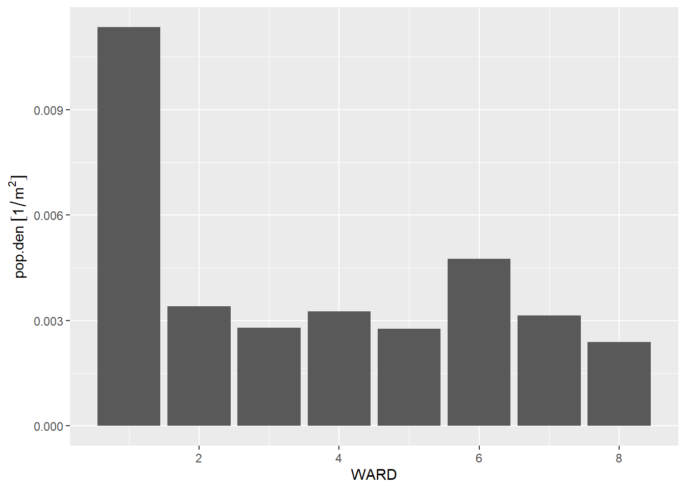
  1. Make a bar chart that shows the population density (people / area) by ward. You may wish to use st_area() to find the area of each ward. Population is already in the ward dataframe.

Answer:

# load library units so command doesnt get mad at me
library(units)
udunits database from C:/Users/lbrooks/AppData/Local/R/win-library/4.2/units/share/udunits/udunits2.xml
# load dc ward shapefile
dc.wards <- st_read("H:/pppa_data_viz/2019/tutorial_data/lecture05/Ward_from_2012/Ward_from_2012.shp")
Reading layer `Ward_from_2012' from data source 
  `H:\pppa_data_viz\2019\tutorial_data\lecture05\Ward_from_2012\Ward_from_2012.shp' 
  using driver `ESRI Shapefile'
Simple feature collection with 8 features and 82 fields
Geometry type: POLYGON
Dimension:     XY
Bounding box:  xmin: -77.1198 ymin: 38.79164 xmax: -76.90915 ymax: 38.99597
Geodetic CRS:  WGS 84
# look at the variables
str(dc.wards)
Classes 'sf' and 'data.frame':  8 obs. of  83 variables:
 $ OBJECTID  : num  1 2 3 4 5 6 7 8
 $ WARD      : num  8 6 7 2 1 5 3 4
 $ NAME      : chr  "Ward 8" "Ward 6" "Ward 7" "Ward 2" ...
 $ REP_NAME  : chr  "Trayon White, Sr." "Charles Allen" "Vincent Gray" "Jack Evans" ...
 $ WEB_URL   : chr  "http://dccouncil.us/council/trayon-white-sr" "http://dccouncil.us/council/charles-allen" "http://dccouncil.us/council/vincent-gray" "http://dccouncil.us/council/jack-evans" ...
 $ REP_PHONE : chr  "(202) 724-8045" "(202) 724-8072" "(202) 724-8068" "(202) 724-8058" ...
 $ REP_EMAIL : chr  "twhite@dccouncil.us" "callen@dccouncil.us" "vgray@dccouncil.us" "jevans@dccouncil.us" ...
 $ REP_OFFICE: chr  "1350 Pennsylvania Ave, Suite 400, NW 20004" "1350 Pennsylvania Ave, Suite 406, NW 20004" "1350 Pennsylvania Ave, Suite 406, NW 20004" "1350 Pennsylvania Ave, Suite 106, NW 20004" ...
 $ WARD_ID   : chr  "8" "6" "7" "2" ...
 $ LABEL     : chr  "Ward 8" "Ward 6" "Ward 7" "Ward 2" ...
 $ AREASQMI  : num  11.94 6.22 8.81 8.68 2.54 ...
 $ Shape_Leng: num  28714 24158 22345 29546 12925 ...
 $ Shape_Area: num  30965852 16064917 22818183 22492798 6567941 ...
 $ POP_2000  : num  74049 70867 69987 63455 71747 ...
 $ POP_2010  : num  73662 76238 71748 76645 74462 ...
 $ POP_2011_2: num  81133 84290 73290 77645 82859 ...
 $ POP_BLACK : chr  "75259" "29909" "69005" "6817" ...
 $ POP_NATIVE: chr  "110" "295" "219" "213" ...
 $ POP_ASIAN : chr  "310" "3573" "225" "7640" ...
 $ POP_HAWAII: chr  "12" "40" "17" "30" ...
 $ POP_OTHER_: chr  "711" "1233" "1211" "2496" ...
 $ TWO_OR_MOR: chr  "872" "2529" "908" "2875" ...
 $ NOT_HISPAN: chr  "79843" "79000" "70987" "69529" ...
 $ HISPANIC_O: chr  "1290" "5290" "2303" "8116" ...
 $ POP_MALE  : chr  "35573" "40411" "33916" "39214" ...
 $ POP_FEMALE: chr  "45560" "43879" "39374" "38431" ...
 $ AGE_0_5   : chr  "7879" "4779" "5230" "2173" ...
 $ AGE_5_9   : chr  "7061" "2747" "4485" "1110" ...
 $ AGE_10_14 : chr  "5963" "2235" "4333" "571" ...
 $ AGE_15_17 : chr  "3596" "1088" "2944" "486" ...
 $ AGE_18_19 : chr  "2945" "1370" "2162" "6200" ...
 $ AGE_20    : chr  "1800" "794" "1347" "3363" ...
 $ AGE_21    : chr  "1748" "724" "1107" "3485" ...
 $ AGE_22_24 : chr  "4070" "4596" "3170" "6463" ...
 $ AGE_25_29 : chr  "6306" "13427" "5036" "12614" ...
 $ AGE_30_34 : chr  "5951" "12512" "5083" "10475" ...
 $ AGE_35_39 : chr  "4617" "8052" "4154" "6491" ...
 $ AGE_40_44 : chr  "4873" "5474" "5166" "4175" ...
 $ AGE_45_49 : chr  "4429" "4524" "4794" "3445" ...
 $ AGE_50_54 : chr  "4978" "4350" "5715" "3413" ...
 $ AGE_55_59 : chr  "5001" "4724" "5272" "3248" ...
 $ AGE_60_61 : chr  "1578" "1830" "1716" "1447" ...
 $ AGE_65_66 : chr  "1011" "1518" "1254" "1214" ...
 $ AGE_67_69 : chr  "1211" "1596" "1680" "1325" ...
 $ AGE_70_74 : chr  "1904" "2167" "2370" "1763" ...
 $ AGE_75_79 : chr  "1026" "1522" "1719" "764" ...
 $ AGE_80_84 : chr  "634" "816" "1290" "724" ...
 $ AGE_85_PLU: chr  "432" "958" "1142" "863" ...
 $ MEDIAN_AGE: chr  "29.3" "33.9" "37" "30.9" ...
 $ UNEMPLOYME: chr  "22.9" "6.3" "19.1" "3.7" ...
 $ TOTAL_HH  : chr  "29470" "40100" "29266" "38870" ...
 $ FAMILY_HH : chr  "17747" "15110" "15574" "9071" ...
 $ PCT_FAMILY: chr  "60.2205632846963" "37.6807980049875" "53.2153352012574" "23.3367635708773" ...
 $ NONFAMILY_: chr  "11723" "24990" "13692" "29799" ...
 $ PCT_NONFAM: chr  "39.7794367153037" "62.3192019950125" "46.7846647987426" "76.6632364291227" ...
 $ PCT_BELOW_: chr  "37.7" "12.5" "27.2" "13.4" ...
 $ PCT_BELO_1: chr  "35.3" "9.6" "23.6" "4.7" ...
 $ PCT_BELO_2: chr  "10.8" "4.5" "8.9" "10.1" ...
 $ PCT_BELO_3: chr  "38.8" "25.7" "28" "33.2" ...
 $ PCT_BELO_4: chr  "54.1" "13.9" "12.8" "26" ...
 $ PCT_BELO_5: chr  "21.6" "11.6" "5.3" "23.5" ...
 $ PCT_BELO_6: chr  "0" "0" "0" "0" ...
 $ PCT_BELO_7: chr  "51.2" "10.7" "19.7" "12.6" ...
 $ PCT_BELO_8: chr  "36.4" "6.2" "20" "10.3" ...
 $ POP_25_PLU: chr  NA NA NA NA ...
 $ POP_25_P_1: chr  "1858" "1785" "2259" "1743" ...
 $ POP_25_P_2: chr  "2614" "25882" "3309" "28509" ...
 $ MARRIED_CO: chr  NA NA NA NA ...
 $ MALE_HH_NO: chr  "1886" "944" "1682" "458" ...
 $ FEMALE_HH_: chr  "11653" "4157" "9499" "754" ...
 $ MEDIAN_HH_: chr  "30910" "94343" "39165" "100388" ...
 $ PER_CAPITA: chr  "17596" "58354" "22917" "72388" ...
 $ PCT_BELO_9: chr  "36.3" "6.3" "22.9" "13.5" ...
 $ PCT_BELO10: chr  "10.8" "4.5" "8.9" "10.1" ...
 $ NO_DIPLOMA: chr  "5958" "3128" "6002" "988" ...
 $ DIPLOMA_25: chr  "18736" "7079" "18683" "2381" ...
 $ NO_DEGREE_: chr  "10975" "6643" "10800" "2980" ...
 $ ASSOC_DEGR: chr  "2149" "1852" "2569" "940" ...
 $ BACH_DEGRE: chr  "3781" "19588" "4890" "16253" ...
 $ MED_VAL_OO: chr  "229900" "573200" "238900" "623500" ...
 $ Shape_Le_1: num  28714 24158 22345 29546 12925 ...
 $ Shape_Ar_1: num  30965852 16064917 22818183 22492798 6567941 ...
 $ geometry  :sfc_POLYGON of length 8; first list element: List of 1
  ..$ : num [1:3792, 1:2] -77 -77 -77 -77 -77 ...
  ..- attr(*, "class")= chr [1:3] "XY" "POLYGON" "sfg"
 - attr(*, "sf_column")= chr "geometry"
 - attr(*, "agr")= Factor w/ 3 levels "constant","aggregate",..: NA NA NA NA NA NA NA NA NA NA ...
  ..- attr(*, "names")= chr [1:82] "OBJECTID" "WARD" "NAME" "REP_NAME" ...
# find the area of each ward
dc.wards$area <- st_area(dc.wards)

# find the population density
dc.wards$pop.den <- dc.wards$POP_2010 / dc.wards$area

# plot the population density
denso <- ggplot() +
  geom_col(data = dc.wards,
           mapping = aes(x = WARD, y = pop.den))
print(denso)

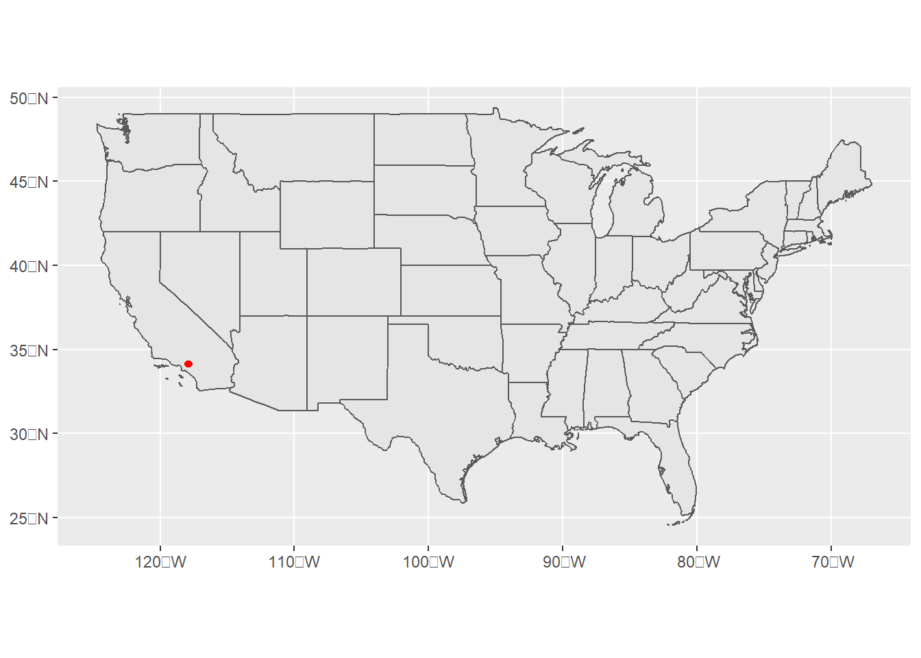
  1. Get two other maps (in shapefile format) not used in this tutorial. Make one ggplot with both of them, and fix the options so that it looks decent.

Answer:

I tried to plot the location of all US Costcos. But the Costco map I found was terrible! It had only two locations. But I plotted nonetheless.

# plotting costco locations in the us

# found costco locations here
# https://www.arcgis.com/home/item.html?id=fea1d6b4a9a04e688b8e61a716150381
costcomap <- st_read("H:/pppa_data_viz/2023/tutorials/answer_programs/tutorial_05/Costco/Costco.shp")
Reading layer `Costco' from data source 
  `H:\pppa_data_viz\2023\tutorials\answer_programs\tutorial_05\Costco\Costco.shp' 
  using driver `ESRI Shapefile'
Simple feature collection with 2 features and 44 fields
Geometry type: POINT
Dimension:     XY
Bounding box:  xmin: -117.9282 ymin: 34.11354 xmax: -117.8284 ymax: 34.13357
Geodetic CRS:  WGS 84
head(costcomap)
Simple feature collection with 2 features and 44 fields
Geometry type: POINT
Dimension:     XY
Bounding box:  xmin: -117.9282 ymin: 34.11354 xmax: -117.8284 ymax: 34.13357
Geodetic CRS:  WGS 84
  X_storefron              address address_li
1        <NA> 1220 W Foothill Blvd       <NA>
2        <NA>  520 N Lone Hill Ave       <NA>
                                                                                                                         category
1 financial,auto rental,general merchandise ,fuel,grocery,travel,auto service,insurance,optometry,hearing,pharmacy,big box stores
2 financial,auto rental,general merchandise ,fuel,grocery,travel,auto service,insurance,optometry,hearing,pharmacy,big box stores
       city       country distributo email_addr fax_number
1     Azusa United States       <NA>       <NA>       <NA>
2 San Dimas United States       <NA>       <NA>       <NA>
               geo_accura last_updat latitude list_id              list_name
1 STREET_ADDRESS: ROOFTOP 2018-06-01 34.13357     129 Costco Wholesale Corp.
2 STREET_ADDRESS: ROOFTOP 2018-06-01 34.11354     129 Costco Wholesale Corp.
  longitude opening_da
1 -117.9282   1-Oct-83
2 -117.8284  16-May-08
                                                       store_hour pharmacy
1   M-F 10:00am - 8:30pm Sat 9:30am - 6:00pm Sun 10:00am - 6:00pm     TRUE
2 M-F 10:00am - 8:30pm Sat. 9:30am - 6:00pm Sun. 10:00am - 6:00pm     TRUE
      pharmacy_p                                      pharmacy_h optical
1 (209) 725-5030 M-F 10:00am-7:00pm SAT 9:30am-6:00pm SUN CLOSED    TRUE
2 (916) 789-1493  M-F 9:00am-7:00pm SAT 9:00am-6:00pm SUN CLOSED    TRUE
  hearing food_court  gas tires country_co             county parent_lis
1    TRUE       TRUE TRUE  TRUE         US Los Angeles County       <NA>
2    TRUE       TRUE TRUE  TRUE         US Los Angeles County       <NA>
  parent_l_1     phone_numb regions sic_code     source_url special_ho
1       <NA> (626) 812-7911    <NA>     5399 www.costco.com       <NA>
2       <NA> (909) 962-5507    <NA>     5399 www.costco.com       <NA>
  special__1 state store_name store_numb store_type              ali unformatte
1       <NA>    CA      Azusa        412       <NA> 129293089-005187       <NA>
2       <NA>    CA  San Dimas       1015       <NA> 129293276-003410       <NA>
  unformat_1 website_ad   zip_code                   geometry
1 6268127911       <NA> 91702-2819 POINT (-117.9282 34.13357)
2 9099625507       <NA> 91773-1725 POINT (-117.8284 34.11354)
dim(costcomap)
[1]  2 45
# get us map
usmap <- st_read("H:/maps/united_states/census2010/states/gz_2010_us_040_00_20m.shp")
Reading layer `gz_2010_us_040_00_20m' from data source 
  `H:\maps\united_states\census2010\states\gz_2010_us_040_00_20m.shp' 
  using driver `ESRI Shapefile'
Simple feature collection with 52 features and 5 fields
Geometry type: MULTIPOLYGON
Dimension:     XY
Bounding box:  xmin: -179.1473 ymin: 17.88481 xmax: 179.7785 ymax: 71.35256
Geodetic CRS:  NAD83
# omit AK, HI, PR
usmap.cont <- usmap[which(!(usmap$STATE %in% c("02","15","72"))),]

# put on top of us map
states <- ggplot() +
  geom_sf(data = usmap.cont) +
  geom_sf(data = costcomap, color = "red")

states