my.seq <- seq(from = 1, to = 11, by = 2)
my.seq
[1] 1 3 5 7 9 11Answer:
Let the height of the bars be \(x_i\), where \(i\) is the index of the \(N\) groups, and \(\sum_{i=1}^N x_i = Z\). If the bar were the share of the total, rather than the group’s total, it would be \(\frac{x_i}{N}\). In other words, either in levels or shares, the bars are simply scaled by a different denominator, keeping their relative position the same.
Answer:
The income histogram looks wacky when the bins are narrow for multiple reasons
Answer:
Answer:
my.seq <- seq(from = 1, to = 11, by = 2)
my.seq[1] 1 3 5 7 9 11# load library
library(tidyverse)── Attaching packages ─────────────────────────────────────── tidyverse 1.3.1 ──✔ ggplot2 3.3.6 ✔ purrr 0.3.4
✔ tibble 3.1.7 ✔ dplyr 1.0.9
✔ tidyr 1.2.0 ✔ stringr 1.4.0
✔ readr 2.1.2 ✔ forcats 0.5.1── Conflicts ────────────────────────────────────────── tidyverse_conflicts() ──
✖ dplyr::filter() masks stats::filter()
✖ dplyr::lag() masks stats::lag()# load the data
# data are created in
# /groups/brooksgrp/pppa_dataviz/r_programs/2021/acsinv03.R
block.groups <- readRDS("h:/pppa_data_viz/2021/tutorial_data/tutorial_04/acs5_bg_dmv_2019_20210202.rds")
names(block.groups) [1] "NAME" "B01001_001E" "B17017_001E" "B17017_002E" "B19013_001E"
[6] "B19057_001E" "B19057_002E" "B25003_001E" "B25003_002E" "B11007_001E"
[11] "B11007_003E" "B25057_001E" "B25058_001E" "B25059_001E" "B25076_001E"
[16] "B25077_001E" "B25079_001E" "B25107_001E" "B25107_002E" "B25107_003E"
[21] "B25107_004E" "B25107_005E" "B25107_006E" "B25107_007E" "B25107_008E"
[26] "B25107_009E" "B25107_010E" "B25107_011E" "state" "county"
[31] "tract" "block.group" "acs" head(block.groups$B25077_001E)[1] 558000 614100 206400 282400 354900 240600summary(block.groups$B25077_001E) Min. 1st Qu. Median Mean 3rd Qu. Max.
-666666666 280350 396650 -42124085 587300 2000001 # get rid of super-low value in 25th percentile distribution
block.groups$p25 <- ifelse(test = block.groups$B25077_001E > 0,
yes = block.groups$B25077_001E,
no = NA)
# make a distribution by state of 25th p of housing value
h1 <- ggplot() +
geom_density(data = block.groups,
mapping = aes(x = p25, y = ..density.., color = as.factor(state))) +
labs(x="25th percentile of housing value",
y="share of block groups")
h1Warning: Removed 228 rows containing non-finite values (stat_density).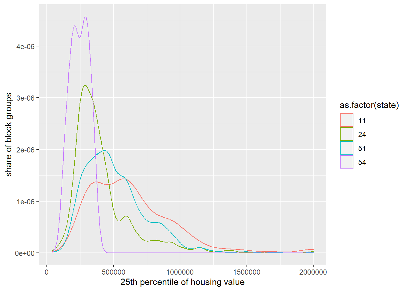
Answer:
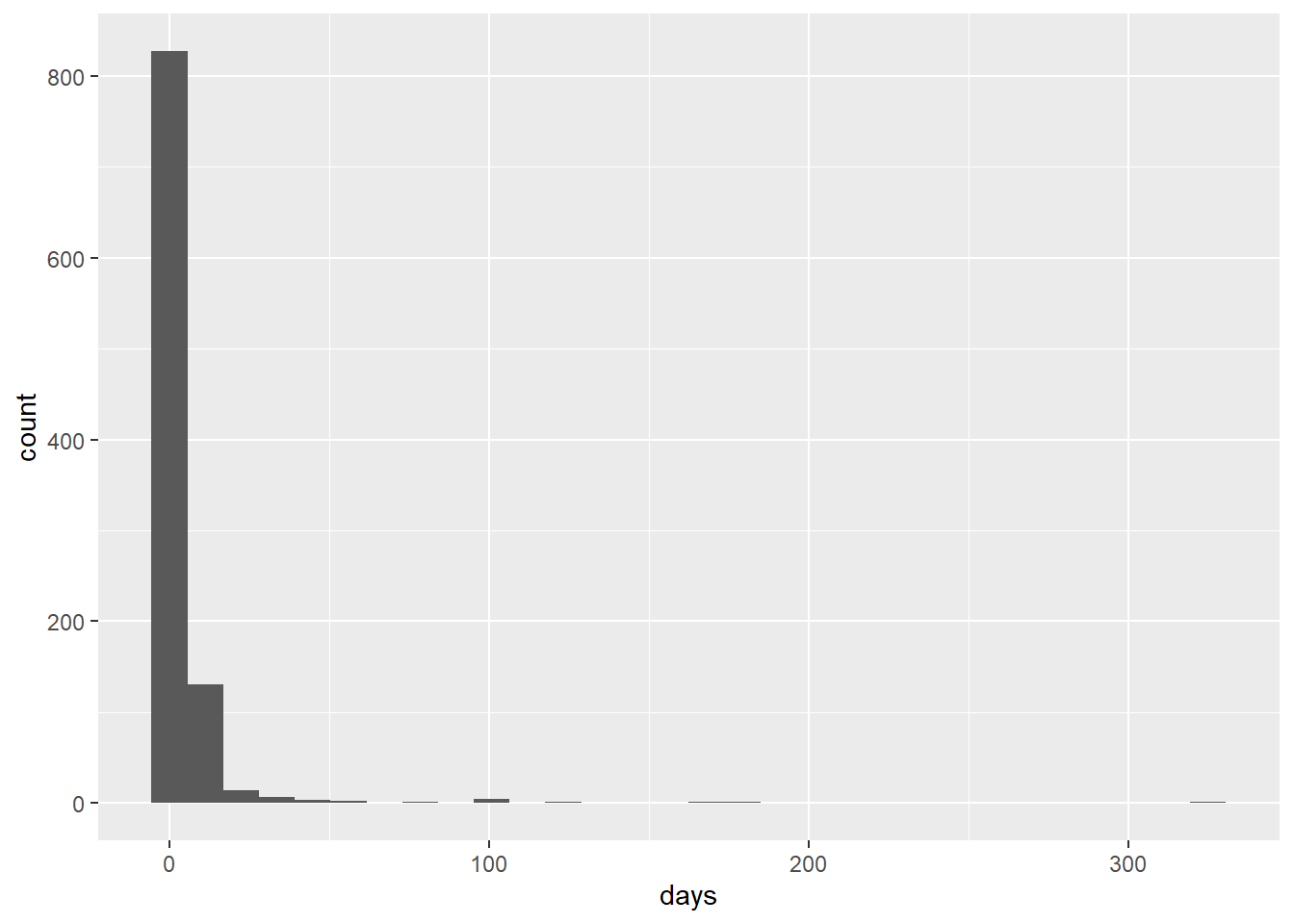
Here is one example, using 311 data from the city of Los Angeles.
# location of la's 311 data for 2022
# https://data.lacity.org/City-Infrastructure-Service-Requests/MyLA311-Service-Request-Data-2022/i5ke-k6by
three11 <- "https://data.lacity.org/resource/i5ke-k6by.csv"

# load the data
la3 <- read_csv(three11)
Rows: 1000 Columns: 34
── Column specification ────────────────────────────────────────────────────────
Delimiter: ","
chr (26): SRNumber, CreatedDate, UpdatedDate, ActionTaken, Owner, RequestTyp...
dbl (8): HouseNumber, ZipCode, Latitude, Longitude, TBMPage, TBMRow, CD, NC
ℹ Use `spec()` to retrieve the full column specification for this data.
ℹ Specify the column types or set `show_col_types = FALSE` to quiet this message.str(la3)spec_tbl_df [1,000 × 34] (S3: spec_tbl_df/tbl_df/tbl/data.frame)
$ SRNumber : chr [1:1000] "1-2154996101" "1-2154995181" "1-2154996311" "1-2154996331" ...
$ CreatedDate : chr [1:1000] "01/01/2022 12:08:14 AM" "01/01/2022 12:15:59 AM" "01/01/2022 12:24:31 AM" "01/01/2022 12:24:38 AM" ...
$ UpdatedDate : chr [1:1000] "01/03/2022 10:39:18 PM" "01/01/2022 01:06:13 PM" "01/03/2022 12:21:42 AM" "01/03/2022 09:37:09 AM" ...
$ ActionTaken : chr [1:1000] "SR Created" "SR Created" "SR Created" "SR Created" ...
$ Owner : chr [1:1000] "LASAN" "LASAN" "LASAN" "LASAN" ...
$ RequestType : chr [1:1000] "Bulky Items" "Dead Animal Removal" "Bulky Items" "Metal/Household Appliances" ...
$ Status : chr [1:1000] "Closed" "Closed" "Cancelled" "Cancelled" ...
$ RequestSource : chr [1:1000] "Self Service" "Call" "Self Service" "Self Service" ...
$ CreatedByUserOrganization: chr [1:1000] "Self Service_SAN" "LASAN" "Self Service" "Self Service_SAN" ...
$ MobileOS : chr [1:1000] NA NA NA NA ...
$ Anonymous : chr [1:1000] "N" "N" "N" "N" ...
$ AssignTo : chr [1:1000] "WLA" "HB" "EV" "WV" ...
$ ServiceDate : chr [1:1000] "01/03/2022 12:00:00 AM" NA "01/05/2022 12:00:00 AM" "01/04/2022 12:00:00 AM" ...
$ ClosedDate : chr [1:1000] "01/03/2022 02:58:20 PM" "01/01/2022 01:06:13 PM" "01/03/2022 12:21:40 AM" "01/03/2022 09:37:08 AM" ...
$ AddressVerified : chr [1:1000] "Y" "Y" "Y" "Y" ...
$ ApproximateAddress : chr [1:1000] "N" "N" "N" "N" ...
$ Address : chr [1:1000] "4776 S LA VILLA MARINA, 90292" "HOOVER ST AT IMPERIAL HWY, 90044" "4144 N TUJUNGA AVE, 91604" "10118 N LURLINE AVE, 91311" ...
$ HouseNumber : num [1:1000] 4776 NA 4144 10118 17101 ...
$ Direction : chr [1:1000] "S" NA "N" "N" ...
$ StreetName : chr [1:1000] "LA VILLA MARINA" NA "TUJUNGA" "LURLINE" ...
$ Suffix : chr [1:1000] NA NA "AVE" "AVE" ...
$ ZipCode : num [1:1000] 90292 90044 91604 91311 91344 ...
$ Latitude : num [1:1000] 34 33.9 34.1 34.3 34.3 ...
$ Longitude : num [1:1000] -118 -118 -118 -119 -119 ...
$ Location : chr [1:1000] "(33.9812287953, -118.433950454)" "(33.930968583, -118.286997573)" "(34.1436314704, -118.378844267)" "(34.2540709722, -118.584098582)" ...
$ TBMPage : num [1:1000] 672 704 562 500 481 594 501 501 501 501 ...
$ TBMColumn : chr [1:1000] "C" "B" "J" "C" ...
$ TBMRow : num [1:1000] 7 6 5 4 6 6 2 2 2 2 ...
$ APC : chr [1:1000] "West Los Angeles APC" "South Los Angeles APC" "South Valley APC" "North Valley APC" ...
$ CD : num [1:1000] 11 8 2 12 12 13 12 12 12 12 ...
$ CDMember : chr [1:1000] "Mike Bonin" "Marqueece Harris-Dawson" "Paul Krekorian" "John Lee" ...
$ NC : num [1:1000] 70 90 27 99 4 38 118 118 118 118 ...
$ NCName : chr [1:1000] "Del Rey" "Harbor Gateway North" "Studio City" "Chatsworth" ...
$ PolicePrecinct : chr [1:1000] "PACIFIC" "SOUTHEAST" "NORTH HOLLYWOOD" "DEVONSHIRE" ...
- attr(*, "spec")=
.. cols(
.. SRNumber = col_character(),
.. CreatedDate = col_character(),
.. UpdatedDate = col_character(),
.. ActionTaken = col_character(),
.. Owner = col_character(),
.. RequestType = col_character(),
.. Status = col_character(),
.. RequestSource = col_character(),
.. CreatedByUserOrganization = col_character(),
.. MobileOS = col_character(),
.. Anonymous = col_character(),
.. AssignTo = col_character(),
.. ServiceDate = col_character(),
.. ClosedDate = col_character(),
.. AddressVerified = col_character(),
.. ApproximateAddress = col_character(),
.. Address = col_character(),
.. HouseNumber = col_double(),
.. Direction = col_character(),
.. StreetName = col_character(),
.. Suffix = col_character(),
.. ZipCode = col_double(),
.. Latitude = col_double(),
.. Longitude = col_double(),
.. Location = col_character(),
.. TBMPage = col_double(),
.. TBMColumn = col_character(),
.. TBMRow = col_double(),
.. APC = col_character(),
.. CD = col_double(),
.. CDMember = col_character(),
.. NC = col_double(),
.. NCName = col_character(),
.. PolicePrecinct = col_character()
.. )
- attr(*, "problems")=<externalptr> # --- calculate the length of time from start to close
# start date
la3$start.date <- as.Date(x = substr(la3$CreatedDate, start = 1, stop = 10), format = "%m/%d/%Y")
# stop date
la3$stop.date <- as.Date(x = substr(la3$ClosedDate, start = 1, stop = 10), format = "%m/%d/%Y")
# number of days between these two
la3$days <- la3$stop.date - la3$start.date
# double-check it
table(la3$days)
  0   1   2   3   4   5   6   7   8   9  10  11  12  13  17  18  19  24  25  32
 61  45 234 191 142 154  74  29   4  10   5   4   3   2   2   1   1   4   6   1
 36  37  40  43  44  45  54  59  78  96  97 101 120 163 174 325
  5   1   1   1   1   1   1   1   1   1   2   2   1   1   1   1
# make a histogram
la.hist <- ggplot() +
geom_histogram(data = la3,
mapping = aes(x = days))
la.histDon't know how to automatically pick scale for object of type difftime. Defaulting to continuous.
`stat_bin()` using `bins = 30`. Pick better value with `binwidth`.Warning: Removed 5 rows containing non-finite values (stat_bin).